Generalized Linear & Linear Mixed Models

glm() and glmer() are extensions of lm() and lmer() models that support non-gaussian outcome variables and support the same methods and attributes. They can be used to estimate modes like logistic regression for binary data and poisson regression for count data.

GLMMs share the same list of methods and attributes available to LMMs.

While these models are relatively simple to use in practice, interpreting what parameter estimates mean can be quite tricky based on how complex the model is and what type of family and link functions you use, with the defaults listed here. We highly recommend making using of the model.emmeans() and model.empredict() methods to instead generate marginal estimates to test specific hypotheses of interest. This tutorial will cover some of these approaches.

from pymer4.models import glm, glmer
import polars as pl, polars.selectors as cs
from polars import col
import seaborn as sns
from pymer4 import load_dataset

Logistic regression

The titantic dataset contains observations of passenger survival rates that we can stratify by other predictors such as passenger \(sex\)

We can see that on average only about 19% of male passengers survived

titanic = load_dataset('titanic')
titanic.group_by('sex').agg(col('survived').mean())

shape: (2, 2)

sex	survived
str	f64
"male"	0.188908
"female"	0.742038

Show code cell source Hide code cell source

ax = sns.countplot(data=titanic, x='survived', hue='sex')
ax.set_xticks([0,1],['No', 'Yes'])
sns.despine();

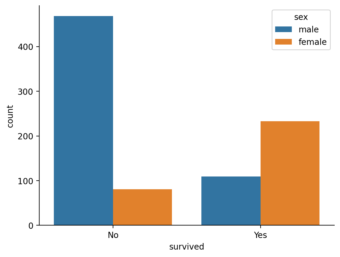
We can model whether the probability of survival is different between sexes with a logistic regression which uses a binomial link-function by default.

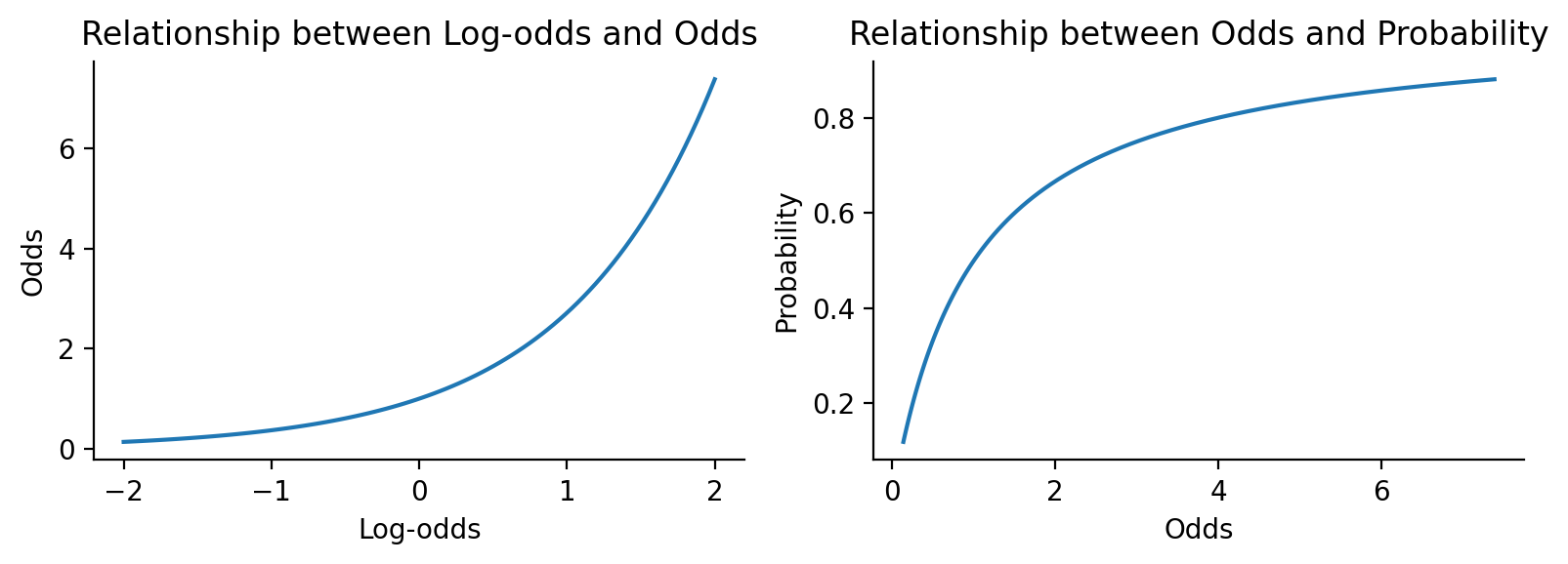
This means that our parameter estimates are on the logit or log-odds scale by default which can be hard be a bit interpret.

\[\begin{split} \begin{align*} p &= probability \\ odds &= \frac{p}{1-p} \\ log\ odds &= logit(p) = ln(\frac{p}{1-p}) \end{align*} \end{split}\]

Show code cell source Hide code cell source

import numpy as np
import matplotlib.pyplot as plt
# Create a range of log-odds values
log_odds = np.linspace(-2, 2, 100)

# Convert to odds and probability
odds = np.exp(log_odds)
prob = odds / (1 + odds)

# Create the plots
fig, (ax1, ax2) = plt.subplots(1, 2, figsize=(8, 3))

# Plot log-odds vs odds
ax1.plot(log_odds, odds)
ax1.set_xlabel('Log-odds')
ax1.set_ylabel('Odds')
ax1.set_title('Relationship between Log-odds and Odds')

# Plot odds vs probability
ax2.plot(odds, prob)
ax2.set_xlabel('Odds')
ax2.set_ylabel('Probability')
ax2.set_title('Relationship between Odds and Probability')

plt.tight_layout()
sns.despine();

log_regress = glm('survived ~ sex', data=titanic, family='binomial')
log_regress.set_factors('sex')
log_regress.fit()
log_regress.params

shape: (2, 2)

term	estimate
str	f64
"(Intercept)"	1.056589
"sexmale"	-2.51371

It can be helpful to make these more interpretable by expontentiating the parameters to be on the odds-scale

log_regress.fit(exponentiate=True)
log_regress.params

shape: (2, 2)

term	estimate
str	f64
"(Intercept)"	2.876543
"sexmale"	0.080967

This shows that Males have .08 odds relative to females of surviving

We can see a full summary view with odds-converted estimates as well

log_regress.summary()

Formula: glm(survived~sex)
Family: binomial (link: default) Number of observations: 891 Confidence intervals: parametric --------------------- Log-likelihood: -458 AIC: 921 | BIC: 931 Residual deviance: 917 | DF: 889 Null deviance: 1186 | DF: 890
	Estimate	SE	CI-low	CI-high	Z-stat	df	p
(Intercept)	2.877	0.371	2.234	3.704	8.191	inf	<.001	***
sexmale	0.081	0.014	0.058	0.112	−15.036	inf	<.001	***
Signif. codes: 0 *** 0.001 ** 0.01 * 0.05 . 0.1

Marginal estimates

In logistic regression, it’s often of interest to pose questions on the probability scale rather than the log-odds or odds scale. For example, what are the respective probabilities of survival for males vs females?

For these kinds of analyses and especially as models include more terms, it’s often a lot easier to use marginal estimates and comparisons rather than trying to interpet .params or .summary() directly

We can do this with the .emmeans() and .empredict() functions which uses type='response' by default to give us probabilities

# Probability of survival by sex
log_regress.emmeans('sex')

shape: (2, 6)

sex	prob	SE	df	asymp_LCL	asymp_UCL
cat	f64	f64	f64	f64	f64
"female"	0.742038	0.02469	inf	0.683113	0.793322
"male"	0.188908	0.016296	inf	0.155122	0.228066

Now we can pose questions in terms of contrasts between these estimates.

This general approach can help make a variety of GLMs much easier to work with. For illustration, contrasting male > female marginal-estimates on the probability-scale, is equivalent to the ratio between the probabilities on the odds-scale, which is what \(sexmale\) represents using .summary(show_odds=True)

log_regress.emmeans('sex', contrasts={'female_minus_male': [-1, 1]})

shape: (1, 9)

contrast	odds_ratio	SE	df	asymp_LCL	asymp_UCL	null	z_ratio	p_value
cat	f64	f64	f64	f64	f64	f64	f64	f64
"female_minus_male"	0.080967	0.013536	inf	0.058346	0.11236	1.0	-15.036107	4.2587e-51

If we switch the default type to 'link' we’ll be comparing estimates on the log-odds scale, which is the same as the untransformed parameter estimate for \(sexmale\)

# Log-odds scale
log_regress.emmeans('sex', type='link')

shape: (2, 6)

sex	emmean	SE	df	asymp_LCL	asymp_UCL
cat	f64	f64	f64	f64	f64
"female"	1.056589	0.128986	inf	0.768114	1.345064
"male"	-1.45712	0.106353	inf	-1.694977	-1.219263

# Contrast is same as untransformed parameter estimate
log_regress.emmeans('sex', contrasts={'female_minus_male': [-1, 1]}, type='link')

shape: (1, 8)

contrast	estimate	SE	df	asymp_LCL	asymp_UCL	z_ratio	p_value
str	f64	f64	f64	f64	f64	f64	f64
"female_minus_male"	-2.51371	0.167178	inf	-2.841373	-2.186046	-15.036107	4.2587e-51

Link functions

For all glm models we can switch to another supported link function. A common one for logistic regression is the 'probit' link function which models probability using the inverse of standard normal cumulative distribution function:

Show code cell source Hide code cell source

import numpy as np
import matplotlib.pyplot as plt
from scipy.stats import norm

# Generate x values from -6 to 6
x = np.linspace(-6, 6, 100)

# Calculate logistic function: 1 / (1 + exp(-x))
logistic = 1 / (1 + np.exp(-x))

# Calculate probit function: standard normal CDF
probit = norm.cdf(x)

# Create plot
plt.figure(figsize=(4,3))
plt.plot(x, logistic, label='Logit', linewidth=2)
plt.plot(x, probit, label='Probit', linewidth=2, linestyle='--')
plt.xlabel('x')
plt.ylabel('Probability')
plt.title('Logit vs Probit Link Functions')
plt.legend()
plt.axvline(x=0, color='k', alpha=0.3)
sns.despine();

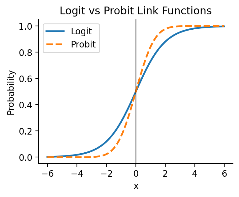
Parameter estimates from a probit model are typically interpreted as the change in z-score of the probability of the outcome under a standard normali distribution.

probit_regress = glm('survived ~ sex', data=titanic, family='binomial', link='probit')
probit_regress.set_factors('sex')
probit_regress.fit()
probit_regress.params

shape: (2, 2)

term	estimate
str	f64
"(Intercept)"	0.649642
"sexmale"	-1.531569

This this scale can be just as hard to interpret as logits/log-odds. And with non-'logit' link functions, there isn’t a consistent way to transform parameter estimates to another scale.

Not to worry, we can use the marginal estimation approach again via .emmeans() to generate predictions and compare probabilities between sexes

probit_regress.emmeans('sex')

shape: (2, 6)

sex	prob	SE	df	asymp_LCL	asymp_UCL
cat	f64	f64	f64	f64	f64
"female"	0.742038	0.02469	inf	0.683927	0.794056
"male"	0.188908	0.016296	inf	0.154647	0.227487

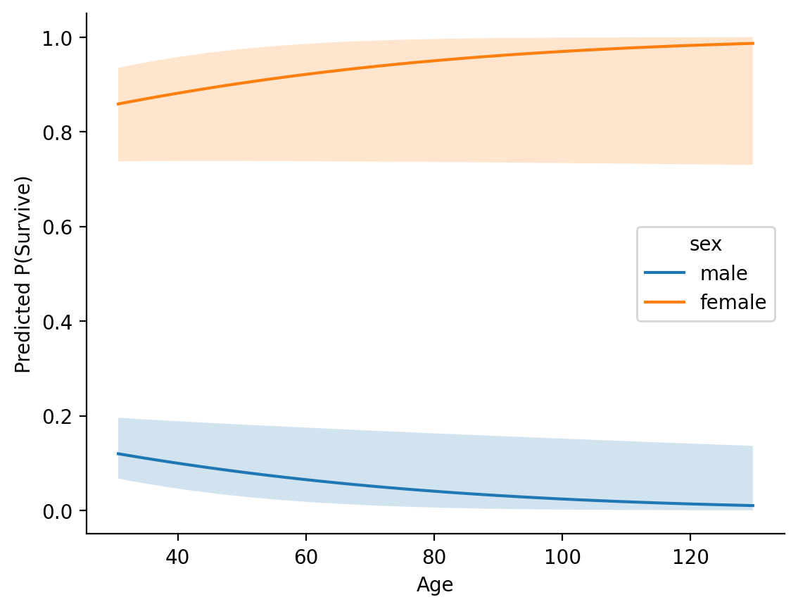
In a more complicated model this can come in very handy for understanding and exploring interactions between predictors:

probit_regress = glm('survived ~ sex * age', data=titanic, family='binomial', link='probit')
probit_regress.set_factors('sex')

# Center age
probit_regress.set_transforms({'age': 'center'})
probit_regress.fit()

# Make predictions for each sex across a range of ages
age_predictions = probit_regress.empredict({
    'sex': ['male', 'female'],
    'age': np.arange(1, 101,1)
    })

# Plot them

Show code cell source Hide code cell source

males = age_predictions.filter(col('sex') == 'male')
females = age_predictions.filter(col('sex') == 'female')

ax =sns.lineplot(data=age_predictions, x='age', y='prob', hue='sex')
ax.fill_between(males['age'], males['asymp_LCL'], males['asymp_UCL'], alpha=0.2)
ax.fill_between(females['age'], females['asymp_LCL'], females['asymp_UCL'],alpha=0.2);
ax.set(xlabel='Age', ylabel='Predicted P(Survive)')
sns.despine();

Multi-level Logistic Regression

We can extend our model to account for the variability across passenger classes by swapping out glm() for glmer() and specifying a random-effects term in this case passenger class

from pymer4.models import glmer

log_lmm = glmer('survived ~ sex + (1 | pclass)', data=titanic, family='binomial')
log_lmm.set_factors('pclass')

# Convert estimates to odds
log_lmm.fit(exponentiate=True, summary=True)

Formula: glmer(survived~sex+(1|pclass))
Family: binomial (link: default) Number of observations: 891 Confidence intervals: parametric --------------------- Log-likelihood: -419 AIC: 845 | BIC: 860 Residual error: 1.0
Random Effects:		Estimate	CI-low	CI-high	SE	Z-stat	df	p
pclass-sd	(Intercept)	0.769
Fixed Effects:
	(Intercept)	3.942	1.576	9.858	1.844	2.933	inf	0.003356	**
	sexmale	0.072	0.050	0.103	0.013	−14.372	inf	<.001	***
Signif. codes: 0 *** 0.001 ** 0.01 * 0.05 . 0.1

This accounts for the variability across each class, nested inside which are multiple observations for each sex. We can explore the odds estimates for each class which captures the variability in the odds of survival across each cluster of observations:

log_lmm.ranef

shape: (3, 2)

level	(Intercept)
str	f64
"1"	2.413829
"2"	1.082862
"3"	0.383755

log_lmm.fixef

shape: (3, 3)

level	(Intercept)	sexmale
str	f64	f64
"1"	9.515432	0.071631
"2"	4.268696	0.071631
"3"	1.512781	0.071631

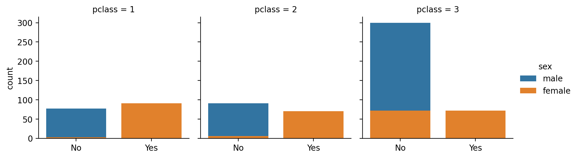
Show code cell source Hide code cell source

grid = sns.FacetGrid(titanic, col='pclass', hue='sex',)
grid.map(sns.countplot, 'survived', order=[0,1])
grid.add_legend()
grid.set_xlabels("")
grid.set_xticklabels(['No', 'Yes'])
sns.despine();

Summary

GLMs and GLMMs support a variety of additional families and link functions for working with different types of data (e.g. family = 'poisson' for count data). You can find a full list here