Categorical Predictors (ANOVA family)#
In the previous tutorial we met the lm() class for estimating univariate and multiple regression models. Here we’ll build upon this by demonstrating how you can work with models that have categorical or factor predictors. All models include the following methods to make it easy to work with categorical predictors which we’ll explore in this tutorial:
Method |
Description |
|---|---|
Set a variable as a factor with alphabetaically sorted levels by default, or specify the exact level ordering; this changes the data-type to categorical/enum |
|
Unset all factor variables to their original datatype |
|
Show any set factors |
|
Encode factor levels using one of the supported coding schemes ( |
|
Show any set contrasts |
|
Calculate a Type-III ANOVA table using |
|
Get a nicely formatted table containing |
|
Compute marginal means/contrasts at specific factor levels |
Basics#
In the previous tutorial we estimated a model with a categorical predictor \(cyl\)
from pymer4.models import lm
from pymer4 import load_dataset
import numpy as np
from polars import col

mtcars = load_dataset('mtcars').select('mpg', 'wt', 'cyl')
model = lm('mpg ~ wt * cyl', data=mtcars)
We specified our factor variable and transformed a continuous variable
model.set_factors({'cyl': ['4', '6', '8']})
model.set_transforms({'wt': 'center'})
We saw that factor variables use treatment contrasts (dummy-coding) by default just like R. This means each parameter represents the difference between the first level and the nth level.
For \(cyl\), that would be \(6-4\) and \(8-4\) as \(4\) is the first level of \(cyl\) based on the order we provided to .set_factors().
model.show_contrasts()
{'cyl': 'contr.treatment'}
Using .set_* methods changes the underlying .data attribute of a model while the coresponding .unset_* methods undo those changes
model.data.head()
| mpg | wt | cyl | wt_orig |
|---|---|---|---|
| f64 | f64 | enum | f64 |
| 21.0 | -0.59725 | "6" | 2.62 |
| 21.0 | -0.34225 | "6" | 2.875 |
| 22.8 | -0.89725 | "4" | 2.32 |
| 21.4 | -0.00225 | "6" | 3.215 |
| 18.7 | 0.22275 | "8" | 3.44 |
# wt has been replaced by its original value previously
# stored in wt_orig
model.unset_transforms()
model.data.head()
| mpg | wt | cyl |
|---|---|---|
| f64 | f64 | i64 |
| 21.0 | 2.62 | 6 |
| 21.0 | 2.875 | 6 |
| 22.8 | 2.32 | 4 |
| 21.4 | 3.215 | 6 |
| 18.7 | 3.44 | 8 |
# cyl is now back to an integer type
model.unset_factors()
model.data.head()
| mpg | wt | cyl | wt_orig |
|---|---|---|---|
| f64 | f64 | i64 | f64 |
| 21.0 | -0.59725 | 6 | 2.62 |
| 21.0 | -0.34225 | 6 | 2.875 |
| 22.8 | -0.89725 | 4 | 2.32 |
| 21.4 | -0.00225 | 6 | 3.215 |
| 18.7 | 0.22275 | 8 | 3.44 |
For factor variables there are several ways to work with .set_contrasts().
The first option is to use any of the default contrasts supported by R
# Mean-center weight again
model.set_transforms({'wt': 'center'})

model.set_factors({'cyl': ['4', '6', '8']})
model.set_contrasts({'cyl': 'contr.sum'})

model.show_contrasts()
{'cyl': 'contr.sum'}
Alternatively we can test a specific hypothesis by using a custom contrast across factor levels with
the order based on the level order set when using
.set_factors()or alphabetically by default.numerical codes that sum-to-zero which will be automatically converted to the contrast matrix expected by R
If we inspect the data we can see that there seems to be an approximately linear trend across levels of \(cyl\)
import seaborn as sns

grid = sns.FacetGrid(data=model.data, palette='Purples', aspect=2)

grid.map(sns.pointplot, 'cyl', 'mpg', color='gray', order=['4','6','8'], alpha=.25, errorbar=None, markersize=10)

grid.map_dataframe(sns.stripplot, 'cyl', 'mpg', order=['4','6','8'], hue='cyl', palette='Purples', legend=True);
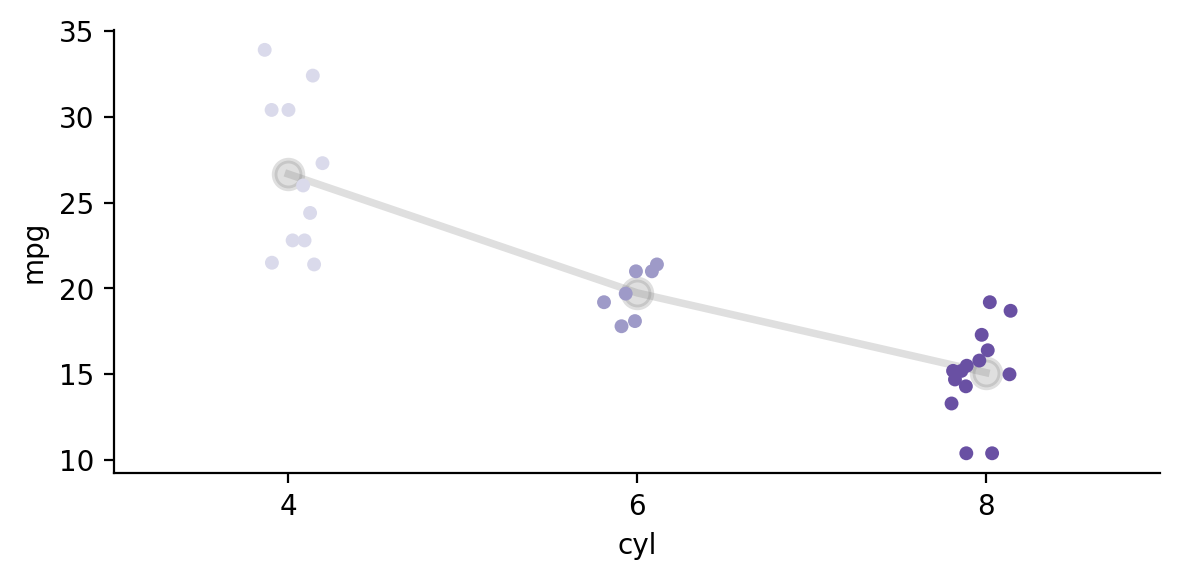
We can test this by specifying a linear contrast across levels of cyl such that 4 < 6 < 8.
The normalize argument simply scales our contrasts for us to match the polynomial used in R:
Now \(cyl1\) below reflects this specific comparison: a linear trend across levels
\(cyl2\) represents an automatically computed orthogonal comparison, in this case a quadratic trend across \(cyl\) levels.
model.set_contrasts({'cyl':[-1, 0, 1]}, normalize=True)
model.fit()
model.params
| term | estimate |
|---|---|
| str | f64 |
| "(Intercept)" | 19.22742 |
| "wt" | -3.539856 |
| "cyl1" | -3.244839 |
| "cyl2" | -0.290422 |
| "wt:cyl1" | 2.442762 |
| "wt:cyl2" | -0.9305 |
We can inspect the .design_matrix after fitting the model to see how our contrast was converted for R and how the second orthogonal contrast was automatically calculated. The code below just grabs and renames the unique rows to make the display easier to see.
The first column is each level of \(cyl\).
The second column is our linear contrast [-1, 0, 1] converted to R’s format of contrast codes.
The third column is the orthogonal contrast auto-calculated for us, which in this case is a quadratic trend
(
    model.design_matrix
    .select('cyl1', 'cyl2')
    .unique(maintain_order=True)
    .with_columns(model.data['cyl'].unique(maintain_order=True))
    .sort('cyl')
    .select('cyl', 'cyl1', 'cyl2')
    .rename({'cyl': 'level', 'cyl1': 'contrast1', 'cyl2': 'contrast2'})
)
| level | contrast1 | contrast2 |
|---|---|---|
| enum | f64 | f64 |
| "4" | -0.707107 | 0.408248 |
| "6" | 0.0 | -0.816497 |
| "8" | 0.707107 | 0.408248 |
Our custom normalized linear contrast is equivalent to using the default contr.poly scheme, which models differences across factor levels as orthogonal polynomials.
Notice that while the parameter names have changes, the estimates are the same as above:
model.set_contrasts({'cyl': 'contr.poly'})
model.fit()
model.params
| term | estimate |
|---|---|
| str | f64 |
| "(Intercept)" | 19.22742 |
| "wt" | -3.539856 |
| "cyl.L" | -3.244839 |
| "cyl.Q" | -0.290422 |
| "wt:cyl.L" | 2.442762 |
| "wt:cyl.Q" | -0.9305 |
Using .set_contrasts() has a direct influence on what a model’s parameter estimates represent. This will influence the output of what you see with .summary(), .params, and .result_fit
This is one way to work with categorical predictors, sometimes called “planned-comparisons”. Later in this tutorial we’ll see an alternative, more general approach using marginal effects estimation.
Common statistical tests are regression#
A variety of common statistical tests that involve comparisons between 2 or more groups, are just linear regression models with categorical predictors:
Often called |
GLM predictor(s) \(X\) |
Example |
|---|---|---|
T-test |
1 two-level categorical |
|
One-way ANOVA |
1 three+ level categorical |
|
ANCOVA |
1 three+ level categorical & 1+ continuous |
|
Moderation |
1 three+ level categorical & 1+ continuous & interaction |
|
Factorial ANOVA |
2 or more two+ level categoricals |
|
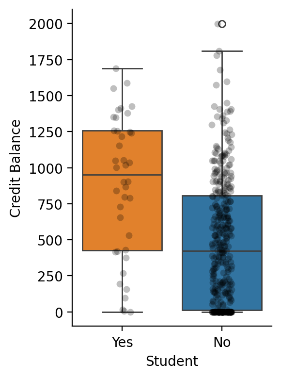
2-levels (t-test)#
Let’s start with a simple example using a categorical variable \(Student\) with 2 levels to compare mean differences in \(Balance\)
Show code cell source
df = load_dataset("credit")

grid = sns.catplot(
    x="Student",
    y="Balance",
    kind="box",
    hue="Student",
    order=["Yes", "No"],
    aspect=0.75,
    height=4,
    data=df.to_pandas(),
)
grid.map(
    sns.stripplot, "Student", "Balance", color="black", alpha=0.25, order=["Yes", "No"]
).set_ylabels('Credit Balance');
After creating the model, we can use .set_factors() treat \(Student\) as a categorical variable. Its levels will be alphabetical by default
model = lm('Balance ~ Student', data=df)

model.set_factors('Student')

model.show_factors()
{'Student': ['No', 'Yes']}
This means that our parameter estimate \(\beta_1\) will reflect \(Student_{Yes} - Student_{No}\)
model.fit(summary=True)
| Formula: lm(Balance~Student) | ||||||||
| Number of observations: 400 Confidence intervals: parametric --------------------- R-squared: 0.0671 R-squared-adj: 0.0647 F(1, 398) = 28.622, p = <.001 Log-likelihood: -3005 AIC: 6016 | BIC: 6028 Residual error: 444.626 |
||||||||
| Estimate | SE | CI-low | CI-high | T-stat | df | p | ||
|---|---|---|---|---|---|---|---|---|
| (Intercept) | 480.369 | 23.434 | 434.300 | 526.439 | 20.499 | 398 | <.001 | *** |
| StudentYes | 396.456 | 74.104 | 250.771 | 542.140 | 5.350 | 398 | <.001 | *** |
| Signif. codes: 0 *** 0.001 ** 0.01 * 0.05 . 0.1 | ||||||||
The t-test on the \(\beta_1\) is equivalent to a two-sample t-test:
Show code cell source
# compare to scipy
from scipy.stats import ttest_ind

student = df.filter(col('Student') == 'Yes').select('Balance')
non_student = df.filter(col('Student') == 'No').select('Balance')

results = ttest_ind(student, non_student)
print(f"Scipy T-test:\ndiff = {student.mean().item() - non_student.mean().item():.3f} t= {results.statistic[0]:.2f} p = {results.pvalue[0]:.3f}")
Scipy T-test:
diff = 396.456 t= 5.35 p = 0.000
3-levels (one-way ANOVA)#
With more than 2 levels of a factor you may want to calculate an F-table, i.e. an ANOVA
penguins = load_dataset('penguins')
Show code cell source
grid = sns.catplot(
    x="species",
    y="body_mass_g",
    kind="box",
    hue="species",
    order=["Adelie", "Chinstrap", "Gentoo"],
    aspect=1,
    height=4,
    data=penguins.to_pandas(),
)
grid.map(
    sns.stripplot,
    "species",
    "body_mass_g",
    color="black",
    alpha=0.25,
    order=["Adelie", "Chinstrap", "Gentoo"],
).set_axis_labels("Species", "Body Mass (g)").figure.suptitle("Penguin Weights", x=.6, fontsize=14);
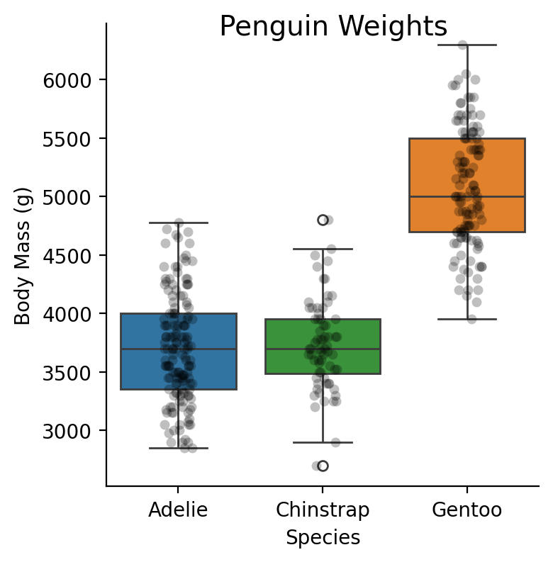
Let’s say we’re interested in the main-effect of \(Species\) on \(Body Mass\)
We can use just .set_factors() and call the .anova() method
model = lm('body_mass_g ~ species', data=penguins)
model.set_factors('species')
model.anova(summary=True)
| ANOVA (Type III tests) | |||||
| model term | df1 | df2 | F_ratio | p_value | |
|---|---|---|---|---|---|
| species | 2 | 339 | 343.626 | <.001 | *** |
| Signif. codes: 0 *** 0.001 ** 0.01 * 0.05 . 0.1 | |||||
Using .anova() is the most convenient way to get omnibus tests on categorical variables (i.e. main effects) especially with more complicated designs. By default it will completely ignore any contrasts you have set (or default contrasts) and use the appropriate ones in the face of both balanced and unbalanced group designs (i.e. orthogonal type-III SS) via emmeans::joint_tests.
This makes it easy to inspect a summary of the hypothesis tests setup by your parameterization without worrying about the correct ANOVA coding-schemes for categorical predictors. Just set your factors with .set_factors() and call .anova()
# Unchanged by ANOVA and determines what we see in .summary()
model.show_contrasts()
{'species': 'contr.treatment'}
# Default treatment contrast with Adelie
# as the reference because alphabetical order
model.params
| term | estimate |
|---|---|
| str | f64 |
| "(Intercept)" | 3700.662252 |
| "speciesChinstrap" | 32.425984 |
| "speciesGentoo" | 1375.354009 |
Marginal Effects Estimation#
Previously we saw how using .set_contrasts() allows us to parameterize our model so we can test specific hypotheses about the levels of a factor variable (e.g. treatment-coding, linear-trend, etc). However, to test a different hypothesis requires re-fitting a new model with new contrasts.
An alternative approach is to compare predictions from a fitted model using predictors set/fixed to particular values. Aggregating and comparing these model-predictions is known as marginal effects estimation. It’s an incredibly powerful general-purpose approach that encompasses traditional techniques like “post-hoc tests” as well as modern approaches like counter-factual estimations. It also makes it easier to reason about more complicated generalized models with interactions, without struggling to potentially mis-interpret parameter estimates alone.
In pymer4 you can compare marginal estimates of each factor levels using .emmeans(), with the order based on how we used .set_factors() and generate arbitrary predictions and comparisons using .empredict()
Using a factor variable as the first argument to .emmeans() provides marginal estimates at each level of the factor while any other model parameters are held at their mean:
model.emmeans('species')
| species | emmean | SE | df | lower_CL | upper_CL |
|---|---|---|---|---|---|
| cat | f64 | f64 | f64 | f64 | f64 |
| "Adelie" | 3700.662252 | 37.619354 | 339.0 | 3610.391084 | 3790.93342 |
| "Chinstrap" | 3733.088235 | 56.059001 | 339.0 | 3598.569406 | 3867.607064 |
| "Gentoo" | 5076.01626 | 41.681876 | 339.0 | 4975.996691 | 5176.035829 |
By using the contrasts argument, you can setup various comparisons of interest with multiple-comparisons correction. Using the 'pairwise' will perform all possible pairwise comparisons. In this case we have only 1 predictor with 3 levels:
model.emmeans('species', contrasts='pairwise', p_adjust='sidak')
| contrast | estimate | SE | df | lower_CL | upper_CL | t_ratio | p_value |
|---|---|---|---|---|---|---|---|
| str | f64 | f64 | f64 | f64 | f64 | f64 | f64 |
| "Adelie - Chinstrap" | -32.425984 | 67.511684 | 339.0 | -194.426598 | 129.574631 | -0.480302 | 0.949888 |
| "Adelie - Gentoo" | -1375.354009 | 56.147971 | 339.0 | -1510.086328 | -1240.621689 | -24.495169 | 0.0 |
| "Chinstrap - Gentoo" | -1342.928025 | 69.856928 | 339.0 | -1510.556273 | -1175.299777 | -19.223978 | 0.0 |
We can also can test a specific comparison using numeric codes in the same order as factor levels
model.emmeans('species', contrasts={'adelie_vs_others': [1, -0.5, -0.5]})
| contrast | estimate | SE | df | lower_CL | upper_CL | t_ratio | p_value |
|---|---|---|---|---|---|---|---|
| str | f64 | f64 | f64 | f64 | f64 | f64 | f64 |
| "adelie_vs_others" | -703.889996 | 51.33433 | 339.0 | -804.863928 | -602.916064 | -13.711877 | 2.3870e-34 |
Compare this to the approach we used before with .set_contrasts(), which allowed us to parameterize a model to test specific comparisons, thus changing what parameter estimates represent.
Using .emmeans() compares model predictions, making it a more generally usefully approach that allows you to ask many questions from a single estimated model.
Parameterizing our model the same way as our marginal estimation above matches the estimated value:
# With auto-solve for other orthogonal contrasts
# speceis1 represents the same comparison as above
model.set_contrasts({'species': [1, -.5, -.5]})
model.fit()
model.params
| term | estimate |
|---|---|
| str | f64 |
| "(Intercept)" | 4169.922249 |
| "species1" | -703.889996 |
| "species2" | 949.593513 |
Multiple predictors (factorial ANOVA)#
Show code cell source
poker = load_dataset('poker')
grid = sns.catplot(
    x="hand",
    y="balance",
    kind="box",
    hue="skill",
    order=["bad", "neutral", "good"],
    hue_order=['average', 'expert'],
    aspect=1,
    height=4,
    data=poker.to_pandas(),
)
grid.map_dataframe(
    sns.stripplot,
    "hand",
    "balance",
    hue='skill',
    palette='dark:black',
    dodge=True,
    alpha=0.25,
    order=["bad", "neutral", "good"],
    hue_order=['average', 'expert'],
).set_axis_labels("Hand Quality", "Money wond ($)").figure.suptitle("Poker Winnings", x=.5, fontsize=14);
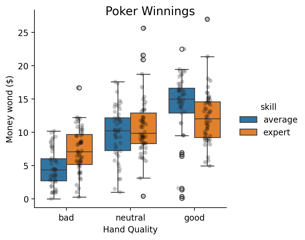
Let’s say we wanted estimate a 2x3 factorial ANOVA. Like before we can use .set_factors() and then call .anova(). Specifying the factor levels isn’t necessary (alphabetic by default), but makes it easier to explore the marginal estimates later.
poker = load_dataset('poker')

model = lm('balance ~ hand * skill', data=poker)

# Set factors
model.set_factors({'hand': ['bad', 'neutral','good'], 'skill':['average', 'expert']})

# Calculate ANOVA
model.anova(summary=True)
| ANOVA (Type III tests) | |||||
| model term | df1 | df2 | F_ratio | p_value | |
|---|---|---|---|---|---|
| hand | 2 | 294 | 79.169 | <.001 | *** |
| skill | 1 | 294 | 2.434 | 0.1198 | |
| hand:skill | 2 | 294 | 7.083 | <.001 | *** |
| Signif. codes: 0 *** 0.001 ** 0.01 * 0.05 . 0.1 | |||||
More Marginal Effects Estimation#
Main effect of skill#
Like before, we can unpack the F-test results using comparison between marginal means.
The F-test result tells are there’s no main-effect of skill, which we can verify by calculating the difference or contrast between each level of skill while averaging over levels of hand.
Notice the p-value is the same and that \(F=t^2\)
skill_contrast = [1, -1]
model.emmeans('skill', contrasts={'avg_vs_expert': skill_contrast})
R messages:
NOTE: Results may be misleading due to involvement in interactions
| contrast | estimate | SE | df | lower_CL | upper_CL | t_ratio | p_value |
|---|---|---|---|---|---|---|---|
| str | f64 | f64 | f64 | f64 | f64 | f64 | f64 |
| "avg_vs_expert" | -0.724333 | 0.464243 | 294.0 | -1.637994 | 0.189328 | -1.560246 | 0.119778 |
We can verify the estimate matches what would have gotten had we calculated the ANOVA cell means ourselves:
average = model.data.filter(col('skill') == 'average').select('balance')
expert = model.data.filter(col('skill') == 'expert').select('balance')
average.mean() - expert.mean()
| balance |
|---|
| f64 |
| -0.724333 |
Main effect of hand#
The F-test for hand indicates a main effect but it doesn’t tell us why.
In the figure above, it looks like there’s an increasing linear trend as we go from bad -> neutral -> good.
Let’s test that, while averaging over levels of skill
# Specified in the order of the factor levels, which we set above
hand_contrast = [-1, 0, 1]
model.emmeans('hand', contrasts={'linear_trend':hand_contrast})
R messages:
NOTE: Results may be misleading due to involvement in interactions
| contrast | estimate | SE | df | lower_CL | upper_CL | t_ratio | p_value |
|---|---|---|---|---|---|---|---|
| str | f64 | f64 | f64 | f64 | f64 | f64 | f64 |
| "linear_trend" | 7.0849 | 0.568579 | 294.0 | 5.965899 | 8.203901 | 12.460706 | 6.6673e-29 |
We can again verify this estimate matches what we would have gotten through manual calculation:
bad = model.data.filter(col("hand") == "bad").select("balance").mean().item()
neutral = model.data.filter(col("hand") == "neutral").select("balance").mean().item()
good = model.data.filter(col("hand") == "good").select("balance").mean().item()

np.dot([bad, neutral, good], hand_contrast)
np.float64(7.084900000000006)
Moderated by skill#
Both the printed message from the previous contrast, as well as the F-test on the interaction tells us that this trend is going to vary depending upon which level of skill we look at.
We can use by to subset out contrast for each level of skill to see how they differ
model.emmeans("hand", by="skill", contrasts={"linear_trend": hand_contrast})
| contrast | skill | estimate | SE | df | lower_CL | upper_CL | t_ratio | p_value |
|---|---|---|---|---|---|---|---|---|
| cat | cat | f64 | f64 | f64 | f64 | f64 | f64 | f64 |
| "linear_trend" | "average" | 9.211 | 0.804093 | 294.0 | 7.628493 | 10.793507 | 11.455148 | 2.2922e-25 |
| "linear_trend" | "expert" | 4.9588 | 0.804093 | 294.0 | 3.376293 | 6.541307 | 6.166951 | 2.2960e-9 |
It does look like the trend is steeper for average players vs expert players. Let’s test that specific interaction by using interaction which allow us to declare a comparison for the by="skill" variable, in the same way that contrasts lets us decare a comparison for the "hand" variable
skill_contrast = [1, -1]

model.emmeans(
    "hand",
    by="skill",
    contrasts={"linear_trend": hand_contrast},
    interaction={"avg_vs_expert": skill_contrast},
)
| contrast | estimate | SE | df | lower_CL | upper_CL | t_ratio | p_value |
|---|---|---|---|---|---|---|---|
| str | f64 | f64 | f64 | f64 | f64 | f64 | f64 |
| "avg_vs_expert" | 4.2522 | 1.137159 | 294.0 | 2.014197 | 6.490203 | 3.73932 | 0.000222 |
Since skill only has 2 levels, we could have used pairwise instead:
model.emmeans(
    "hand",
    by="skill",
    contrasts={"linear_trend": hand_contrast},
    interaction="pairwise",
)
| contrast | estimate | SE | df | lower_CL | upper_CL | t_ratio | p_value |
|---|---|---|---|---|---|---|---|
| str | f64 | f64 | f64 | f64 | f64 | f64 | f64 |
| "linear_trend average - linear_… | 4.2522 | 1.137159 | 294.0 | 2.014197 | 6.490203 | 3.73932 | 0.000222 |
This is a little more work to calculate manually but matches our estimate:
Show code cell source
bad_a = (
    model.data.filter(col("hand") == "bad", col("skill") == "average")
    .select("balance")
    .mean()
    .item()
)
neutral_a = (
    model.data.filter(col("hand") == "neutral", col("skill") == "average")
    .select("balance")
    .mean()
    .item()
)
good_a = (
    model.data.filter(col("hand") == "good", col("skill") == "average")
    .select("balance")
    .mean()
    .item()
)
bad_e = (
    model.data.filter(col("hand") == "bad", col("skill") == "expert")
    .select("balance")
    .mean()
    .item()
)
neutral_e = (
    model.data.filter(col("hand") == "neutral", col("skill") == "expert")
    .select("balance")
    .mean()
    .item()
)
good_e = (
    model.data.filter(col("hand") == "good", col("skill") == "expert")
    .select("balance")
    .mean()
    .item()
)
# Toggle code above to see calculations
np.dot([bad_a, neutral_a, good_a], hand_contrast) - np.dot(
    [bad_e, neutral_e, good_e], hand_contrast
)
np.float64(4.252199999999995)
Comparison to re-parameterizing model#
Alternatively, we can parameterize our regression model such that our coefficients reflect the comparisons we want, so called “planned comparisons”. Rather than use .anova(), we’ll now want to use .fit() and inspect the \(k-1\) parameters for each \(k\) level categorical predictor.
Let’s change the default treatment-coding to the comparisons we care about:
# Reuse from before
# linear contrast across levels of hand
# average - expert for skill
model.set_contrasts({'hand': hand_contrast, 'skill': skill_contrast})
model.show_contrasts()
{'hand': array([-1, 0, 1]), 'skill': array([ 1, -1])}
Now the estimates capture what we care about.
Since hand has 3 levels, we need 2 parameters to fully capture it
hand1 = linear contrast (bad < neutral < good) averaged over skill
hand2 = automatically computed quadratic contrast averaged over skill
Since skill had 2 levels, we just need 1 parameter to capture it
skill1 = average - expert difference averaged over hand
The first interaction parameter reflect linear trend difference we calculated above:
hand1:skill1 = linear contrast average skill - linear contrast expert skill
hand2:skill1 = automatically computed quadratic contrast average skill - quadratic contrast expert skill
model.fit(summary=True)
| Formula: lm(balance~hand*skill) | ||||||||
| Number of observations: 300 Confidence intervals: parametric --------------------- R-squared: 0.3731 R-squared-adj: 0.3624 F(5, 294) = 34.988, p = <.001 Log-likelihood: -840 AIC: 1694 | BIC: 1720 Residual error: 4.02 |
||||||||
| Estimate | SE | CI-low | CI-high | T-stat | df | p | ||
|---|---|---|---|---|---|---|---|---|
| (Intercept) | 9.771 | 0.232 | 9.315 | 10.228 | 42.096 | 294 | <.001 | *** |
| hand1 | 7.085 | 0.569 | 5.966 | 8.204 | 12.461 | 294 | <.001 | *** |
| hand2 | −0.704 | 0.402 | −1.496 | 0.087 | −1.752 | 294 | 0.08083 | . |
| skill1 | −0.724 | 0.464 | −1.638 | 0.189 | −1.560 | 294 | 0.1198 | |
| hand1:skill1 | 4.252 | 1.137 | 2.014 | 6.490 | 3.739 | 294 | <.001 | *** |
| hand2:skill1 | 0.344 | 0.804 | −1.238 | 1.927 | 0.428 | 294 | 0.6687 | |
| Signif. codes: 0 *** 0.001 ** 0.01 * 0.05 . 0.1 | ||||||||
All pairwise comparisons#
Though not encouraged, we can also calculate the pairwise comparisons between every combination of hand and skill
model.emmeans(['hand', 'skill'], contrasts='pairwise', p_adjust='bonferroni')
| contrast | estimate | SE | df | lower_CL | upper_CL | t_ratio | p_value |
|---|---|---|---|---|---|---|---|
| str | f64 | f64 | f64 | f64 | f64 | f64 | f64 |
| "bad average - neutral average" | -5.2572 | 0.804093 | 294.0 | -7.636816 | -2.877584 | -6.538053 | 4.1276e-9 |
| "bad average - good average" | -9.211 | 0.804093 | 294.0 | -11.590616 | -6.831384 | -11.455148 | 3.4383e-24 |
| "bad average - bad expert" | -2.7098 | 0.804093 | 294.0 | -5.089416 | -0.330184 | -3.37001 | 0.012781 |
| "bad average - neutral expert" | -6.2628 | 0.804093 | 294.0 | -8.642416 | -3.883184 | -7.788655 | 1.7546e-12 |
| "bad average - good expert" | -7.6686 | 0.804093 | 294.0 | -10.048216 | -5.288984 | -9.536961 | 8.7939e-18 |
| … | … | … | … | … | … | … | … |
| "good average - neutral expert" | 2.9482 | 0.804093 | 294.0 | 0.568584 | 5.327816 | 3.666493 | 0.004376 |
| "good average - good expert" | 1.5424 | 0.804093 | 294.0 | -0.837216 | 3.922016 | 1.918187 | 0.840836 |
| "bad expert - neutral expert" | -3.553 | 0.804093 | 294.0 | -5.932616 | -1.173384 | -4.418645 | 0.00021 |
| "bad expert - good expert" | -4.9588 | 0.804093 | 294.0 | -7.338416 | -2.579184 | -6.166951 | 3.4440e-8 |
| "neutral expert - good expert" | -1.4058 | 0.804093 | 294.0 | -3.785416 | 0.973816 | -1.748306 | 1.0 |
With continuous predictor(s) (e.g. ANCOVA/moderation)#
Show code cell source
grid = sns.lmplot(
    x="flipper_length_mm",
    y="body_mass_g",
    hue="species",
    hue_order=["Adelie", "Chinstrap", "Gentoo"],
    aspect=1,
    height=4,
    data=penguins.to_pandas(),
)
grid.set_axis_labels("Flipper Length", "Body Mass (g)").figure.suptitle("Penguin Weights", x=.6, fontsize=14);
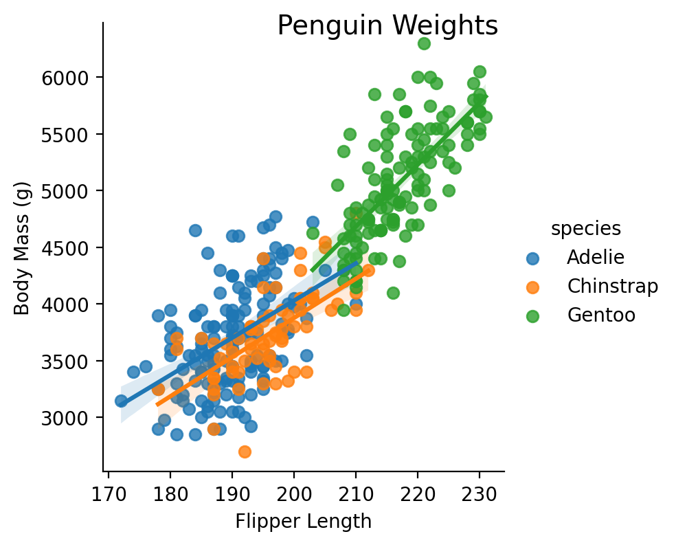
Models with mixed continuous and factor models work exactly the same.
Here we explore whether there’s an interaction between species and flipper length, i.e. whether a penguin’s species changes the relationship between flipper length and body mass.
model = lm('body_mass_g ~ species * flipper_length_mm', data=penguins)

# Categorical
model.set_factors('species')
model.set_contrasts({'species':'contr.sum'})

# Continuous
model.set_transforms({'flipper_length_mm': 'center'})

# Calculate ANOVA
model.anova(summary=True)
| ANOVA (Type III tests) | |||||
| model term | df1 | df2 | F_ratio | p_value | |
|---|---|---|---|---|---|
| species | 2 | 336 | 3.934 | 0.02047 | * |
| flipper_length_mm | 1 | 336 | 168.292 | <.001 | *** |
| species:flipper_length_mm | 2 | 336 | 5.532 | 0.004327 | ** |
| Signif. codes: 0 *** 0.001 ** 0.01 * 0.05 . 0.1 | |||||
While we could try to understand these relationships just based on the estimated parameters, it’s much easier to unpack them using marginal effects estimation
model.params
| term | estimate |
|---|---|
| str | f64 |
| "(Intercept)" | 4052.294709 |
| "species1" | 8.254155 |
| "species2" | -143.169979 |
| "flipper_length_mm" | 40.675862 |
| "species1:flipper_length_mm" | -7.844172 |
| "species2:flipper_length_mm" | -6.102468 |
Even more Marginal Effects Estimation#
\(flipper\_length\_mm\) above is the slope of flipper_length_mm averaged over species since we used sum (deviation) coding
model.emmeans('flipper_length_mm')
R messages:
NOTE: Results may be misleading due to involvement in interactions
| flipper_length_mm_trend | SE | df | lower_CL | upper_CL |
|---|---|---|---|---|
| f64 | f64 | f64 | f64 | f64 |
| 40.675862 | 3.135487 | 336.0 | 34.508204 | 46.84352 |
\(species1\) is the first parameter of our sum (deviation) coding which represents factor levels as a differences from the grand-mean, when flipper_length_mm is held at its mean.
species_means = model.emmeans('species').select('emmean')
grand_mean = species_means.mean().item()
adelie_mean = species_means[0]
adelie_mean - grand_mean
R messages:
NOTE: Results may be misleading due to involvement in interactions
| emmean |
|---|
| f64 |
| 8.254155 |
\(species2\) is the difference between the next factor level (Chinstrap) and the grand-mean
species_means[1] - grand_mean
| emmean |
|---|
| f64 |
| -143.169979 |
With marginal estimation we can also ask questions about our continuous predictor. For example, passing using flipper_length_mm as our first variable and species as our by variable we can see how the slope of \(flipper length\) varies across \(species\)
model.emmeans('flipper_length_mm', by='species')
| species | flipper_length_mm_trend | SE | df | lower_CL | upper_CL |
|---|---|---|---|---|---|
| cat | f64 | f64 | f64 | f64 | f64 |
| "Adelie" | 32.83169 | 4.627184 | 336.0 | 21.727836 | 43.935543 |
| "Chinstrap" | 34.573394 | 6.348364 | 336.0 | 19.339225 | 49.807563 |
| "Gentoo" | 54.622502 | 5.173874 | 336.0 | 42.206757 | 67.038247 |
Like before, we can use the contrasts argument to specify a test across levels of our by variable, i.e. a test across the different slopes above.
Here we test whether the relationship between flipper_length and weight gets stronger across species: Adelie < Chinstrap < Gentoo, i.e. that the slope increases
model.emmeans("flipper_length_mm", by="species", contrasts={"linear": [-1, 0, 1]}, normalize=True)
| contrast | estimate | SE | df | lower_CL | upper_CL | t_ratio | p_value |
|---|---|---|---|---|---|---|---|
| str | f64 | f64 | f64 | f64 | f64 | f64 | f64 |
| "linear" | 15.408431 | 4.908146 | 336.0 | 5.753865 | 25.062997 | 3.139359 | 0.001843 |
Counter-factual estimates & comparisons#
We can also calculate marginal means at arbitrary values of flipper_length_mm using the at keyword and passing in 1 or more values. Let’s test a hypothetical question: how would species differ in weight if we were to observe a very short flipper_length_mm of 150mm?
We never actually observe this value of flipper_length_mm but can we can use the model to generate a counter-factual comparisons to get an answer:
model.emmeans('species', at={'flipper_length_mm': 150}, contrasts='pairwise')
R messages:
NOTE: Results may be misleading due to involvement in interactions
| contrast | estimate | SE | df | lower_CL | upper_CL | t_ratio | p_value |
|---|---|---|---|---|---|---|---|
| str | f64 | f64 | f64 | f64 | f64 | f64 | f64 |
| "Adelie - Chinstrap" | 240.103356 | 348.902095 | 336.0 | -597.157041 | 1077.363752 | 0.688168 | 0.868765 |
| "Adelie - Gentoo" | 982.82199 | 396.284903 | 336.0 | 31.857066 | 1933.786915 | 2.480089 | 0.040319 |
| "Chinstrap - Gentoo" | 742.718635 | 456.726766 | 336.0 | -353.288637 | 1838.725907 | 1.626177 | 0.282721 |
For even more control we can use .empredict() to generate predictions for arbitrary combinations of our predictors. This allows us to ask very specific questions like:
How much would an Adelie penguin weigh if it had a flipper length of 210mm?
.empredict() (and .emmeans()) will automatically handle transformations from .set_transforms() and return values of the predictor on the transformed scale along with predictions and uncertainty
model.empredict({'flipper_length_mm': 210, 'species': 'Adelie'})
| species | flipper_length_mm | prediction | SE | df | lower_CL | upper_CL |
|---|---|---|---|---|---|---|
| cat | f64 | f64 | f64 | f64 | f64 | f64 |
| "Adelie" | 9.084795 | 4358.818046 | 97.537889 | 336.0 | 4166.956202 | 4550.67989 |
Using the special 'data' value allows us to easily reference all the observed values for a predictor. For example, we can generate unit-level predictions using all observed flipper lengths only for Chinstrap and Gentoo penguins
model.empredict({'flipper_length_mm': 'data', 'species': ['Chinstrap', 'Gentoo']}).head()
| species | flipper_length_mm | prediction | SE | df | lower_CL | upper_CL |
|---|---|---|---|---|---|---|
| cat | f64 | f64 | f64 | f64 | f64 | f64 |
| "Chinstrap" | -19.915205 | 3220.588515 | 104.285847 | 336.0 | 3015.453103 | 3425.723926 |
| "Gentoo" | -19.915205 | 3099.392229 | 190.185526 | 336.0 | 2725.287906 | 3473.496551 |
| "Chinstrap" | -14.915205 | 3393.455484 | 76.869652 | 336.0 | 3242.249081 | 3544.661886 |
| "Gentoo" | -14.915205 | 3372.504738 | 164.781292 | 336.0 | 3048.371798 | 3696.637678 |
| "Chinstrap" | -5.915205 | 3704.616029 | 45.244783 | 336.0 | 3615.617307 | 3793.61475 |