Quickstart

This notebook demos the core features of pymer4 models, which are intentionally designed to be similar to their R counter-parts with numerous quality-of-life features and enhancements.

Installation

First follow the installation guide to setup pymer4 using conda or Google Collab

Picking a model

pymer4 provides 4 types of models that share a consistent API:

Model	Description
lm()	linear regression fit via ordinary-least-squares (OLS)
glm()	generalized linear models (e.g logistic regression) fit via maximum-likelihood-estimate (MLE)
lmer()	linear-mixed / multi-level models
glmer()	geneneralized linear-mixed / multi-level models

Loading data

All models work with polars Dataframes. If you are coming from pandas you can easily convert between libraries, but you should also seriously consider switching:

• pandas -> polars: import polars as pl; pl.DataFrame(pd_frame)

• polars -> pandas: pl_frame.to_pandas()

Included are a number of datasets accessible with the load_dataset() function. Let’s load the popular mtcars dataset:

from pymer4 import load_dataset

# Load the dataset
cars = load_dataset('mtcars')

# Get the columns we want
df = cars.select('mpg', 'cyl', 'wt')

# Show the first 5 rows
df.head()

shape: (5, 3)

mpg	cyl	wt
f64	i64	f64
21.0	6	2.62
21.0	6	2.875
22.8	4	2.32
21.4	6	3.215
18.7	8	3.44

Fitting a linear model

Let’s estimate the following univariate regression model:

\[ mpg \sim \beta_0 + \beta_1 * wt \]

We can use lm class to create a model which simply requires a formula and some data

from pymer4.models  import lm

# Initialize model
model = lm('mpg ~ wt', data=df)

model

pymer4.models.lm(fitted=False, formula=mpg~wt)

Models make a copy of the input dataframe and store it in their .data attribute. As we’ll soon see, this dataframe will be augmented with additional columns after fitting a model or applying any variable transforms

model.data.head()

shape: (5, 3)

mpg	cyl	wt
f64	i64	f64
21.0	6	2.62
21.0	6	2.875
22.8	4	2.32
21.4	6	3.215
18.7	8	3.44

We can use the .fit() method to estimate parameters and inferential statistics which are stored as inside a model object and can be accessed with a variety of methods (model.method()) or attributes (model.attribute).

model.fit()

Calling .fit() will create the following attributes for all models:

• .params: parameter estimates (coefficients) for model terms

• .result_fit: summary style table of parameter estimates and inferential stats

• .result_fit_stat: model quality-of-fit statistics

• augment .data: add fit and residual columns to the dataframe

# Inspect parameter estimates
model.params

shape: (2, 2)

term	estimate
str	f64
"(Intercept)"	37.285126
"wt"	-5.344472

We can see all this information quickly using the .summary() method (or by using .fit(summary=True)) which returns a nicely formatted great table

model.summary()

Formula: lm(mpg~wt)
Number of observations: 32 Confidence intervals: parametric --------------------- R-squared: 0.7528 R-squared-adj: 0.7446 F(1, 30) = 91.375, p = <.001 Log-likelihood: -80 AIC: 166 | BIC: 170 Residual error: 3.046
	Estimate	SE	CI-low	CI-high	T-stat	df	p
(Intercept)	37.285	1.878	33.450	41.120	19.858	30	<.001	***
wt	−5.344	0.559	−6.486	−4.203	−9.559	30	<.001	***
Signif. codes: 0 *** 0.001 ** 0.01 * 0.05 . 0.1

We can also print a more basic R-style summary

model.summary(pretty=False)

Coefficients:
            Estimate Std. Error t value Pr(>|t|)    
(Intercept)  37.2851     1.8776  19.858  < 2e-16 ***
wt           -5.3445     0.5591  -9.559 1.29e-10 ***
---
Signif. codes:  0 ‘***’ 0.001 ‘**’ 0.01 ‘*’ 0.05 ‘.’ 0.1 ‘ ’ 1

Residual standard error: 3.046 on 30 degrees of freedom
Multiple R-squared:  0.7528,	Adjusted R-squared:  0.7446 
F-statistic: 91.38 on 1 and 30 DF,  p-value: 1.294e-10

Or get a nice report

model.report()

We fitted a linear model (estimated using OLS) to predict mpg with wt (formula:
mpg ~ wt). The model explains a statistically significant and substantial
proportion of variance (R2 = 0.75, F(1, 30) = 91.38, p < .001, adj. R2 = 0.74).
The model's intercept, corresponding to wt = 0, is at 37.29 (95% CI [33.45,
41.12], t(30) = 19.86, p < .001). Within this model:

  - The effect of wt is statistically significant and negative (beta = -5.34, 95%
CI [-6.49, -4.20], t(30) = -9.56, p < .001; Std. beta = -0.87, 95% CI [-1.05,
-0.68])

Standardized parameters were obtained by fitting the model on a standardized
version of the dataset. 95% Confidence Intervals (CIs) and p-values were
computed using a Wald t-distribution approximation.

You can always directly access this information from the model attributes:

# summary table
model.result_fit

shape: (2, 8)

term	estimate	std_error	conf_low	conf_high	t_stat	df	p_value
str	f64	f64	f64	f64	f64	i64	f64
"(Intercept)"	37.285126	1.877627	33.4505	41.119753	19.857575	30	8.2418e-19
"wt"	-5.344472	0.559101	-6.486308	-4.202635	-9.559044	30	1.2940e-10

# Quality-of-fit statistics
model.result_fit_stats

shape: (1, 12)

r_squared	adj_r_squared	sigma	statistic	p_value	df	logLik	AIC	BIC	deviance	df_residual	nobs
f64	f64	f64	f64	f64	f64	f64	f64	f64	f64	i64	i64
0.752833	0.744594	3.045882	91.375325	1.2940e-10	1.0	-80.014714	166.029429	170.426637	278.321938	30	32

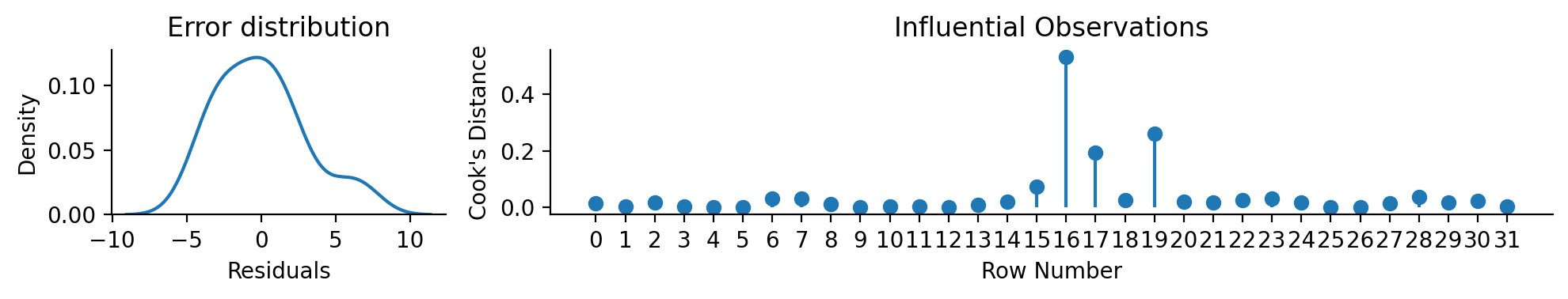
If we now inspect the .data attribute of the model we’ll see several new columns that have been appended to the original data. These contain model predictions, residuals, and statistics per observation

model.data.head()

shape: (5, 9)

mpg	cyl	wt	fitted	resid	hat	sigma	cooksd	std_resid
f64	i64	f64	f64	f64	f64	f64	f64	f64
21.0	6	2.62	23.282611	-2.282611	0.043269	3.067494	0.013274	-0.766168
21.0	6	2.875	21.91977	-0.91977	0.035197	3.093068	0.001724	-0.307431
22.8	4	2.32	24.885952	-2.085952	0.058376	3.072127	0.015439	-0.705752
21.4	6	3.215	20.10265	1.29735	0.03125	3.088268	0.003021	0.432751
18.7	8	3.44	18.900144	-0.200144	0.032922	3.097722	0.000076	-0.066819

Which makes visual model inspection very easy

Show code cell source Hide code cell source

import matplotlib.pyplot as plt
import seaborn as sns

# Setup subplots
f = plt.figure(figsize=(10, 2))
gs = f.add_gridspec(1, 2, width_ratios=[1, 3])
left, right = f.add_subplot(gs[0]), f.add_subplot(gs[1])

# We can just use the 'resid' column for the first plot
left = sns.kdeplot(x='resid', data=model.data, ax=left)
left.set(xlabel='Residuals', title="Error distribution")

# And the 'cooksd' column to create a plot of observation influence
right.stem(model.data['cooksd'], basefmt=' ', label='Cook\'s Distance')
right.set(xlabel='Row Number', ylabel='Cook\'s Distance', title="Influential Observations", xticks=range(model.data.height))

sns.despine()
plt.tight_layout();

Categorical predictors and predictor transforms

Let’s say we wanted to extend our model to estimate a multiple regression including an interaction with a categorical-predictor \(cyl\)

\[mpg \sim \beta_0 + \beta_1 * wt + \beta_2 * cyl + \beta_3 * wt * cyl\]

For these situations, pymer4 provides a common set of tools for manipulating the types and values of predictors:

• .set/unset/show_factors(): treat variables as factors

• .set/show_contrasts(): specify contrast coding schemes for factors

• .set/unset/show_transforms(): apply a common transform to numerical predictors (e.g. centering)

We can use .set_factors() to treat \(cyl\) as a factor with levels in the specified order. Omitting a specific order will use alphabetical order by default.
We can check any currently set factor variables with .show_factors()

# Initialize model
model = lm('mpg ~ wt * cyl', data=df)

# Set cyl as a factor with levels in this order
model.set_factors({'cyl': ['4', '6', '8']})

model.show_factors()

{'cyl': ['4', '6', '8']}

Factor variables adhere to a contrast coding scheme and using treatment contrasts (dummy-coding) by default just like R. We can use .show_contrasts() to view the currently set coding scheme:

model.show_contrasts()

{'cyl': 'contr.treatment'}

For continuous predictors, we can apply common transformations using .set_transforms() (e.g. 'center', 'scale', 'zscore', 'rank').

We’ll mean-center \(wt\) so difference between levels of \(cyl\) are interpretable when \(wt\) is equal to its mean.

# Mean center wt
model.set_transforms({'wt': 'center'})

model.show_transforms()

{'wt': 'center'}

Manipulating factors and transforms changes the .data attribute of a model. We can see that cyl is now an enum type which is how polars treats categorical variables. We also have a new column wt_orig that contains the original values of \(wt\), while wt contains the transformed (mean-centered) values:

model.data.head()

shape: (5, 4)

mpg	cyl	wt	wt_orig
f64	enum	f64	f64
21.0	"6"	-0.59725	2.62
21.0	"6"	-0.34225	2.875
22.8	"4"	-0.89725	2.32
21.4	"6"	-0.00225	3.215
18.7	"8"	0.22275	3.44

This makes it easy to quickly adjust predictor types and values without having to create a new model.

Caling .fit() now re-estimates the same formula on the same .data - which now has different types/values. So our parameter estimates now represent the comparisons specified by our contrasts and transformations:

• mean-centered \(wt\)

• treatment-coded \(cyl\) with \(4\) as the reference level

model.fit(summary=True)

Formula: lm(mpg~wt*cyl)
Number of observations: 32 Confidence intervals: parametric --------------------- R-squared: 0.8616 R-squared-adj: 0.8349 F(5, 26) = 32.362, p = <.001 Log-likelihood: -70 AIC: 155 | BIC: 165 Residual error: 2.449
	Estimate	SE	CI-low	CI-high	T-stat	df	p
(Intercept)	21.403	1.466	18.390	24.416	14.601	26	<.001	***
wt	−5.647	1.359	−8.442	−2.853	−4.154	26	<.001	***
cyl6	−1.939	1.756	−5.549	1.671	−1.104	26	0.2797
cyl8	−4.589	1.751	−8.188	−0.990	−2.621	26	0.01446	*
wt:cyl6	2.867	3.117	−3.541	9.275	0.920	26	0.3662
wt:cyl8	3.455	1.627	0.110	6.799	2.123	26	0.04344	*
Signif. codes: 0 *** 0.001 ** 0.01 * 0.05 . 0.1

ANOVA tables

With more than 2 levels of a categorical predictor, you may be interested in an omnibus F-test across all factor levels, i.e. an ANOVA style table. To make this as easy and valid as possible (e.g. handling unbalanced designs) just create your factors with .set_factors() and use .anova() instead of .fit()

model.anova(summary=True)

ANOVA (Type III tests)
model term	df1	df2	F_ratio	p_value
wt	1	26	10.723	0.002993	**
cyl	2	26	3.951	0.03175	*
wt:cyl	2	26	2.266	0.1239
Signif. codes: 0 *** 0.001 ** 0.01 * 0.05 . 0.1

Just like .fit() the dataframe results of .anova() are accessible via .result_anova

model.result_anova

shape: (3, 5)

model term	df1	df2	F_ratio	p_value
str	f64	f64	f64	f64
"wt"	1.0	26.0	10.723	0.002993
"cyl"	2.0	26.0	3.951	0.031753
"wt:cyl"	2.0	26.0	2.266	0.123857

Tip

You can learn more about working with transforms, factors, contrasts, and ANOVA in the categorical predictors tutorial

Marginal estimates & contrasts

Every model supports the .emmeans() method that takes one or more predictors of the same type and generates marginal estimates while other predictors are held at their means. For example, using \(cyl\) will return the average \(mpg\) for each level of \(cyl\) while holding \(wt\) at its mean.

model.emmeans('cyl')

R messages: 
NOTE: Results may be misleading due to involvement in interactions

shape: (3, 6)

cyl	emmean	SE	df	lower_CL	upper_CL
cat	f64	f64	f64	f64	f64
"4"	21.403304	1.465893	26.0	17.66308	25.143528
"6"	19.464549	0.967159	26.0	16.996845	21.932253
"8"	16.814408	0.95775	26.0	14.370711	19.258106

Passing a continuous predictor \(wt\) to .emmeans() will calculate the average slope of that variable while other variables are held at their means. In this case the slope of \(wt\), while \(cyl\) is held at the grand-mean across factor levels.

This matches the regression parameter estimate for \(wt\) in the output of .summary() above:

model.emmeans('wt')

R messages: 
NOTE: Results may be misleading due to involvement in interactions

shape: (1, 5)

wt_trend	SE	df	lower_CL	upper_CL
f64	f64	f64	f64	f64
-3.539856	1.081023	26.0	-5.76193	-1.317783

Using the by argument allow us to subset the estimates of one predictor by another predictor.
For example, we can unpack the interaction by calculating separate slopes of \(wt\) for each level of \(cyl\)

model.emmeans('wt', by='cyl')

shape: (3, 6)

cyl	wt_trend	SE	df	lower_CL	upper_CL
cat	f64	f64	f64	f64	f64
"4"	-5.647025	1.359498	26.0	-9.115782	-2.178268
"6"	-2.780106	2.805265	26.0	-9.937736	4.377524
"8"	-2.192438	0.894285	26.0	-4.474204	0.089329

We can use the at argument to the reverse: explore the means for each level of \(cyl\) at a specific valued of \(wt\)

model.emmeans('cyl', at={'wt': 3})

R messages: 
NOTE: Results may be misleading due to involvement in interactions

shape: (3, 6)

cyl	emmean	SE	df	lower_CL	upper_CL
cat	f64	f64	f64	f64	f64
"4"	22.63012	1.219839	26.0	19.517702	25.742539
"6"	20.068527	0.9821	26.0	17.562699	22.574354
"8"	17.290715	1.10759	26.0	14.464702	20.116729

Using the contrasts argument, we can test specific comparisons between levels of a predictor.

# linear contrast across factor levels
# (-1 * 4) + (0 * 6) + (1 * 8)
model.emmeans('cyl', contrasts={'linear':[-1, 0, 1]})

R messages: 
NOTE: Results may be misleading due to involvement in interactions

shape: (1, 8)

contrast	estimate	SE	df	lower_CL	upper_CL	t_ratio	p_value
str	f64	f64	f64	f64	f64	f64	f64
"linear"	-4.588896	1.751036	26.0	-8.188202	-0.98959	-2.620675	0.014464

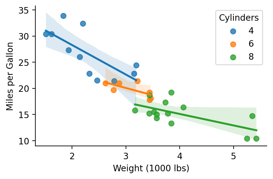
Models also support the .empredict() method for even more control in generating predictions based on specific predictor values.

For example, we though we never observe a 4 cylinder vehicle that weighs more that 4000lbs, we can have the model predict the miles-per-gallon based on the estimated parameters:

Show code cell source Hide code cell source

import seaborn as sns
grid = sns.lmplot(x='wt_orig', y='mpg', hue='cyl', data=model.data, height=3, aspect=1.5, facet_kws={'legend_out': False})
grid.set_axis_labels("Weight (1000 lbs)", "Miles per Gallon")
grid.legend.set_title("Cylinders");

# Predict mpg when weight is 4k, 5k, and 6k
# mean-centering trasnform is appled for us
model.empredict({'wt': [4,5,6], 'cyl': '4'})

shape: (3, 7)

wt	cyl	prediction	SE	df	lower_CL	upper_CL
f64	cat	f64	f64	f64	f64	f64
0.78275	"4"	16.983095	2.444694	26.0	11.957955	22.008235
1.78275	"4"	11.33607	3.763179	26.0	3.600744	19.071395
2.78275	"4"	5.689044	5.103232	26.0	-4.800798	16.178887

Multi-level models

Working with multi-level/mixed-effects models is just as easy using lmer or glmer classes and support the same random-effects formula syntax popularized by lme4.

from pymer4 import load_dataset
from pymer4.models import lmer

sleep = load_dataset('sleep')

# Random intercept, slope, and correlation
lmm_is = lmer('Reaction ~ Days + (Days | Subject)', data=sleep)
lmm_is.fit(summary=True)

Formula: lmer(Reaction~Days+(Days|Subject))
Number of observations: 180 Confidence intervals: parametric --------------------- Log-likelihood: -871 AIC: 1755 | BIC: 1774 Residual error: 25.592
Random Effects:		Estimate	SE	CI-low	CI-high	T-stat	DF	p
Subject-sd	(Intercept)	24.741
Subject-sd	Days	5.922
Subject-cor	(Intercept)	0.066
Residual-sd	Observation	25.592
Fixed Effects:
	(Intercept)	251.405	6.825	237.006	265.804	36.838	17.000	<.001	***
	Days	10.467	1.546	7.206	13.729	6.771	17.000	<.001	***
Signif. codes: 0 *** 0.001 ** 0.01 * 0.05 . 0.1

Multi-level models have the following additional atttributes to make working with random-effects easier:

• .ranef - cluster level deviances

• .ranef_var - cluster level variance-covariances

• .fixef - BLUPs; cluster level coefficients (.params + .ranef)

# Slope and intercept for each Subject
lmm_is.fixef.head()

shape: (5, 3)

level	(Intercept)	Days
str	f64	f64
"308"	253.663656	19.666262
"309"	211.006367	1.847605
"310"	212.444696	5.018429
"330"	275.095724	5.652936
"331"	273.665417	7.397374

# Variance across Subject level slopes and intercepts
lmm_is.ranef_var

shape: (4, 5)

group	term	estimate	conf_low	conf_high
str	str	f64	f64	f64
"Subject"	"sd__(Intercept)"	24.740658	null	null
"Subject"	"cor__(Intercept).Days"	0.065551	null	null
"Subject"	"sd__Days"	5.922138	null	null
"Residual"	"sd__Observation"	25.591796	null	null

And we can generate a summary report:

lmm_is.report()

We fitted a linear mixed model (estimated using REML and nloptwrap optimizer)
to predict Reaction with Days (formula: Reaction ~ Days). The model included
Days as random effects (formula: ~Days | Subject). The model's total
explanatory power is substantial (conditional R2 = 0.80) and the part related
to the fixed effects alone (marginal R2) is of 0.28. The model's intercept,
corresponding to Days = 0, is at 251.41 (95% CI [237.94, 264.87], t(174) =
36.84, p < .001). Within this model:

  - The effect of Days is statistically significant and positive (beta = 10.47,
95% CI [7.42, 13.52], t(174) = 6.77, p < .001; Std. beta = 0.54, 95% CI [0.38,
0.69])

Standardized parameters were obtained by fitting the model on a standardized
version of the dataset. 95% Confidence Intervals (CIs) and p-values were
computed using a Wald t-distribution approximation.

We can refit the model using bootstrapping to get confidence intervals around both fixed and radom effects

lmm_is.fit(conf_method='boot', summary=True)

Formula: lmer(Reaction~Days+(Days|Subject))
Number of observations: 180 Confidence intervals: boot Bootstrap Iterations: 1000 --------------------- Log-likelihood: -871 AIC: 1755 | BIC: 1774 Residual error: 25.592
Random Effects:		Estimate	CI-low	CI-high	SE	T-stat	DF	p
Subject-sd	(Intercept)	24.741	12.073	35.774
Subject-sd	Days	5.922	3.360	8.370
Subject-cor	(Intercept)	0.066	−0.481	0.948
Residual-sd	Observation	25.592	22.746	28.588
Fixed Effects:
	(Intercept)	251.405	237.902	263.832	6.825	36.838	17.000	<.001	***
	Days	10.467	7.362	13.255	1.546	6.771	17.000	<.001	***
Signif. codes: 0 *** 0.001 ** 0.01 * 0.05 . 0.1

Comparing models

pymer4 offers a general-purpose compare() function to compare 2 or more nested models using an F-test or Likelihood-Ratio-Test. This is handy for comparing the random-effects structure of various mixed models

from pymer4.models import compare

# Random intercept only model
lmm_i = lmer('Reaction ~ Days + (1 | Subject)', data=sleep)

# Suggests modeling slopes is worth it
compare(lmm_is, lmm_i)

Analysis of Deviance Table
Model 1: lmer(Reaction~Days+(Days|Subject)) Model 2: lmer(Reaction~Days+(1|Subject))
	AIC	BIC	logLik	npar	-2*log(L)	Chisq	Df	Pr(>Chisq)
1.00	1755.6	1774.8	−871.8	4.00	1.79K
2.00	1794.5	1807.2	−893.2	6.00	1.75K	42.14	2.00	<.001	***
Signif. codes: 0 *** 0.001 ** 0.01 * 0.05 . 0.1

For linear models, compare() performs nested-model comparison, which is a more general purpose approach that can be used to answer the same question as the interaction F-test in the ANOVA table above

# Define model without interaction
add_only = lm('mpg ~ wt + cyl', data=df)
add_only.set_factors({'cyl': ['4', '6', '8']})

# Compare to our original model
compare(model, add_only)

Analysis of Deviance Table
Model 1: lm(mpg~wt*cyl) Model 2: lm(mpg~wt+cyl)
	AIC	BIC	logLik	Res_Df	RSS	Df	Sum of Sq	F	Pr(>F)
1.00	155.5	165.7	−70.7	26.00	155.89
2.00	156.6	164	−73.3	28.00	183.06	−2.00	−27.17	2.27	0.124
Signif. codes: 0 *** 0.001 ** 0.01 * 0.05 . 0.1

Summary and next steps

This quickstart provided an overview of the core functionality when working with models in pymer4. For more in-depth tutorials check out:

• linear regression tutorial which also demonstrates features common to all pymer4 models

• categorical variables tutorial if you’re working with factorial designs or non-numeric predictors

• multi-level models tutorial for repeated-measures or hierarchical data

• generalized linear/multi-level models tutorial for non-gaussian outcome variables (e.g. logistic regression)

• scikit-learn compatible estimators using the skmer class

You can read about the specific arguments and outputs of different model methods on their respective API pages, e.g. lm.fit()

If you’re interested in more advanced functionality, you explore the tidystats module that export many popular R functions from a variety of libraries (and powers pymer4.models !)