Comparing common analysis strategies for repeated measures data
What is this all about?
My hope with this post is to provide a conceptual overview of how to deal with a specific type of dataset commonly encountered in the social sciences (and very common in my own disciplines of experimental psychology and cognitive neuroscience). My goal is not to provide mathematical formalisms, but rather build some intuitions and try to avoid as much jargon as possible. Specifically, I’d like to compare some of the more common analysis strategies one can use and how they vary by situation, ending with some takeaways that hopefully guide your future decision-making. But to do so we need to start at the beginning…
Repeated what?
Datasets come in all different shapes and sizes. In many introductory tutorials, classes, and even real world examples, folks are usually dealing with datasets that are referred to as satisfying the “i.i.d assumption” of many common statistical models. What does this mean in English? It refers to the fact that each data-point is largely independent of other data points in the complete dataset. More specifically, it means that the residuals of a model (i.e. what’s left over that the model can’t explain) are independent of each other and that they all come from the same distribution which has a mean of 0 and a standard deviation of \(\sigma^2\). In other words, knowing something about one error that the model makes tells you little about any other error the model makes, and by extension, knowing something about one data point tells you little about any other datapoint.
However, many types of data contain “repeats” or “replicates” such as measuring the same people over time or under different conditions. These data notably violate this assumption. In these cases, some data points are more similar to each other than other data points. Violations of these assumptions can lead to model estimates that are not as accurate as they could possibly be (Ugrinowitsch et al, 2004). The more insidious issue is that inferences made using these estimates (e.g. computing t-statistics and by extension p-values) can be wildly inaccurate and produce false-positives (Vasey & Thayer, 1987). Let’s try to make this more concrete by considering two different datasets.
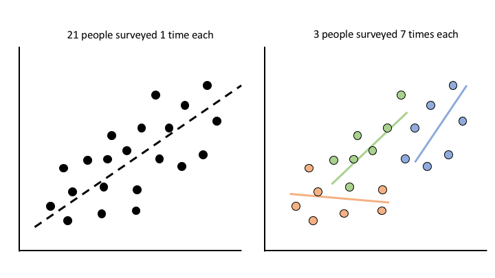
In case 1 (left) we give 21 people a survey 1 time each and try to see if their survey responses share any relationship with some demographic about them. 21 total data points, pretty straightforward. In case 2 (right), we give 3 people a survey 7 times each and do the same thing. 21 total data points again, but this time each data point is not independent of every other. In the first case, each survey response is independent of any other. That is, knowing something about one person’s response tells you little about another person’s response. However, in the second case this is not true. Knowing something about person A’s survey response the first time you survey them tells you a bit more about person A’s survey response the second time you survey them, whereas it does necessarily give you more information about any of person B’s responses. Hence the non-independence. In the most extreme case estimating a model ignoring these dependencies in the data can completely reverse the resulting estimates, a phenomenon known as Simpson’s Paradox.
Analysis Strategies.
So what do we typically do? Well there are a few different analysis “traditions” that have dealt with this in different ways. This isn’t by any means an exhaustive list, but approaches that are reasonably common across many different literatures.
Multi-level models
Like many other researchers in psychology/neuroscience, I was first taught that repeated-measures ANOVAs are the only way to analyze these type of data. However, this has fallen a bit out of practice in favor of the more flexible approach of multi-level/mixed effects modeling (Baayen et al, 2008). I don’t want to focus on why multi-level modeling is often far more preferable, as that’s a different discussion (e.g. better handling of missing data, different numbers of repeats, additional levels of replicates, different numbers of replicates, etc), but suffice to say that it once you start using this approach there’s essentially no reason to ever run a repeated measured ANOVA again. Going into all the details of how these models work is beyond the scope of this post, but I’ll link to a few resources throughout. Conceptually, multi-level modeling simultaneously estimates coefficients that describe a relationship across the entire dataset, as well as within each group of replicates. In our example above, this amounts to estimating the relationship between survey responses and demographics for the entire population of survey respondents, but also the degree to which individual people deviate from these estimates. This has the net effect of “pooling” estimates and their associated errors together and works in a manner not entirely unlike using a prior if you are familiar with Bayesian terminology or regularization/smoothing if machine-learning is more your thing. The result of estimating a model this way means that estimates can “help each other out” such that we can impute values if some of our survey respondents didn’t fill out the survey each time we asked them to, or we can “clean-up” noisy estimates we get from specific individuals by assuming that individuals’ estimates all come from the same population, thereby restricting wonky values they may take on.
In practice using these models can be a bit tricky. This is due to the fact that it’s not immediately obvious how to set these models up for estimation. For example, should we assume that each respondent has a different relationship between their survey results and demographics? Or should we simply assume that their survey results differ on average but vary with their demographics in the same way? Specifically, users have a variety of choices for how to specify what’s referred to as the “random effects” (deviation estimates) part of the model. You may have come across terminology like “random intercepts” or “random slopes.” In our example, this is the difference between allowing a model to learn a unique mean estimate for each individual’s survey responses and learning a unique regression estimate for the relationship between each individual’s survey responses and demographic outcome measure. In many cases, computing the complete set of coefficients one could compute (intercepts, slopes, and the correlations between them for every predictor) (Barr, et al, 2013) leads the model to fail to converge, leaving a user with unreliable estimates. This has lead to suggestions to keep models relatively “simple” with respect to the inference one is trying to make (Bates, et al 2015), or compare different model structures and use a model selection criteria to adjudicate between them before performing inferences (Matuschek et al, 2017). Pretty tricky huh? Try this guide to help you out if you venture down this path or check out this post for a nice visual treatment. Brauer & Curtin, 2018 is a particularly good one-stop-shop for review, theory, practice, estimation issues, and code snippets. There are a ton of resources available if multi-level models have got you excited.
Robust/corrected standard errors
In other academic fields/areas, there is an entirely different tradition for handling these types of data. For example, in some economics disciplines “robust/sandwich/huber-white” standard errors are computed for what is otherwise a standard linear regression model. This lecture provides a nice math-ish overview of what these techniques are, but the general takeaway is that this approach entails computing the regression coefficients in a “typical” manner using ordinary least squares (OLS) regression, but “correcting” the variance of these estimators (i.e. the standard errors) for how heteroscedastic they are. That is, how much their variances differ. There are several ways to account for heteroscedasticicty that incorporate things like small-sample and auto-correlation correction, but another one is to compute these robust estimates with respect to “clusters” or grouping factors in the data. In the example above, clusters would comprise survey respondents and each survey response would comprise a data point within that cluster. Therefore, this approach completely ignores the fact that there are repeated measurements when computing the regression coefficients, but takes the repeated measures data into account when making inferences on these coefficients by adjusting their standard errors. For an overview of this calculation see this presentation and for a more formal treatment see Cameron & Miller, 2015.
Two-stage-regression/summary statistics approach*
Finally, a third approach we can use is what has been sometimes referred to as a two-stage-regression (Gelman, 2005) or the summary statistics approach (Frison & Pocock, 1992; Holmes & Friston, 1998). This approach is routine in the analysis of functional MRI data (Mumford & Nichols, 2009). Conceptually, this looks like fitting a standard OLS regression model to each survey respondent separately, and then fitting a second OLS model to the coefficients from each individual subject’s fit. In the simplest case this equivalent to calculating a one-sample t-test over individuals’ coefficients. You might notice that this approach “feels” similar to the multi-level approach, and in colloquial English, there are in fact multiple levels of modeling going on. However, notice how each first-level model is estimated completely independently of every other model and how their errors or the variance of their estimates are not aggregated in any meaningful way. This means that we lose out on some of the benefits we gain from the formal multi-level modeling framework described above. Yet what we might lose in benefits we gain back in simplicity: there are no additional choices to be made such as choosing an appropriate “random effects” structure. In fact, Gelman, 2005 notes that two-stage-regression can be viewed as a special case of multi-level modeling in which we assume that the distribution from which individual/cluster level coefficients comes has infinite variance.
How do we decide?
Having all these tools at our disposal can sometimes make it tricky to figure out which approach is preferable for what situation and whether there is one approach that is always better than the others (spoiler: there isn’t). To better understand when we might use each approach let’s consider some of the most common situations we might encounter. I’ll refer to these as the “dimensions” along which our data can vary.
Dimension 1: Sample size of units we would like to make inferences about
The most common thing that varies about different datasets is simply their size, i.e. how many observations we’re really dealing with. In the case of non-independent data, an analyst may most often be interested in making inferences about a particular “level” of the data. In our survey example, this is generalizing to “people” rather than specific instances of the survey. So this dimension varies based on how many individuals we sampled, irrespective of how many times we sampled any given individual.
Dimension 2: Sample size of units nested within units we would like to make inferences about
Another dimension in which our repeated-measures data may vary, is how many repeats we’re dealing with. In our example above, this is the number of observations we have about any given individual. Did each person fill out the survey 5 times? 10? 100? This dimension therefore varies based on how often we sample any given individual, irrespective of how many total individuals we sample.
Dimension 3: Variability between units we would like to make inferences about
A key way in which each of these analysis approaches varies is how they handle (or don’t) variability between clusters of replicates. In our example above, this is the variance between individuals. Do different people really respond differently from each other? At one extreme we can treat every individual survey response as entirely independent ignoring the fact that we surveyed individuals multiple times and pretending each survey is totally unique. At the other end, we can assume that the relationship between survey responses and demographics come from a higher-level distribution and specific people’s estimates are instances of this distribution, preserving the fact that each person’s own responses are more similar to each other than they are to anyone else’s responses. I’ll return to this a bit more below.
Simulations can help us build intuitions.
Often in cases like this we can use simulated data, designed to vary in particular ways, to help us gain some insight as to how these things influence our different analysis strategies. So let’s see how that looks. I’m going to be primarily using the pymer4 Python package that I wrote to simulate some data and compare these different models. I wrote this package originally so I could reduce the switch cost I kept experiencing bouncing between R and Python for my work. I quickly realized that my primary need for R was using the fantastic lme4 package for multi-level modeling and so I wrote this Python package as a way to use lme4 from within Python while playing nicely with the rest of the scientific Python stack (e.g. pandas, numpy, scipy, etc). Since then the package has grown quite a bit (Jolly, 2018), including the ability to fit the different types of models discussed above and simulate different kinds of data. Ok let’s get started:
# Import what we need
import pandas as pd
import numpy as np
from pymer4.simulate import simulate_lmm, simulate_lm
from pymer4.models import Lm, Lmer, Lm2
import matplotlib.pyplot as plt
import seaborn as sns
sns.set_context('poster');
sns.set_style("whitegrid")
%matplotlib inline
Starting small
Let’s start out with a single simulated dataset and fit each type of model discussed above. Below I’m generating multi-level data similar to our toy example above. The dataset is comprised of 50 “people” with 50 “replicates” each. For each person, we measured 3 independent variables (e.g. 3 survey questions) and would like to relate them to 1 dependent variable (e.g. 1 demographic outcome).
num_obs_grp = 50
num_grps = 50
num_coef = 3
formula = 'DV ~ IV1 + IV2 + IV3' # Not required for generating data, but just for convenience estimating models below
data, blups, betas = simulate_lmm(num_obs_grp, num_coef, num_grps)
data.head()
| DV | IV1 | IV2 | IV3 | Group | |
|---|---|---|---|---|---|
| 0 | 0.962692 | 0.884919 | -1.027279 | 1.267401 | 1.0 |
| 1 | 0.692995 | -0.034800 | 1.487490 | -0.623623 | 1.0 |
| 2 | -0.227617 | -0.841247 | 0.227976 | -1.411721 | 1.0 |
| 3 | -0.502931 | 1.466788 | -1.332548 | -1.336735 | 1.0 |
| 4 | 2.254925 | 0.675905 | -0.400129 | 0.977755 | 1.0 |
We can see that the overall dataset is generated as described above. Simulating data this way also allows us to generate the best-linear-unbiased-predictions (BLUPs) for each person in our dataset. These are the coefficients for each individual person.
blups.head()
| Intercept | IV1 | IV2 | IV3 | |
|---|---|---|---|---|
| Grp1 | 0.334953 | 0.804446 | 1.273423 | 0.484458 |
| Grp2 | 0.296504 | 0.533969 | 1.499689 | -0.323965 |
| Grp3 | 0.269028 | 0.748626 | 0.826473 | 0.494888 |
| Grp4 | 0.489680 | 0.714883 | 1.073006 | 0.103898 |
| Grp5 | 0.224353 | 0.898960 | 1.171890 | 0.034940 |
Finally, we can also checkout the “true” coefficients that generated these data. These are the “correct answers” we hope that our models can recover. Since these data have been simulated using the addition of noise to each individual’s data (\((\mu=0,\sigma^2=1)\), and with variance across individuals (pymer4’s default is \(\sigma^2=0.25\)) we don’t expect perfect recovery of these parameters, but something pretty close (we’ll explore this more below).
print(f"True betas: {betas}")
# Regression  coefficients for intercept, IV1, IV2, and IV3
True betas: [0.18463772 0.78093358 0.97054762 0.45977883]
Evaluating performance
Ok time to evaluate some modeling strategies. For each model type I’ll fit the model to the data as described, and then compute 3 metrics:
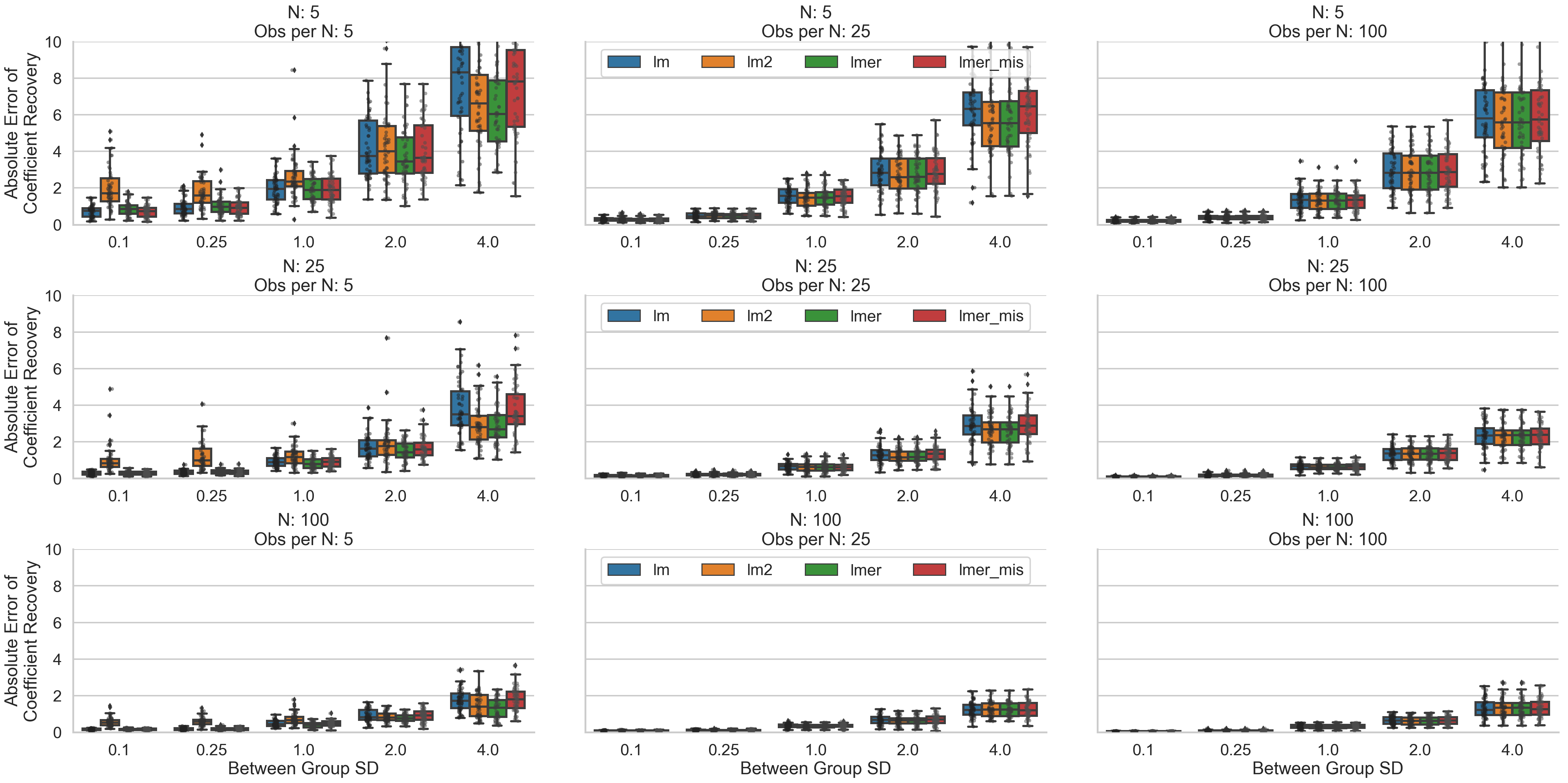
- Absolute Error of Coefficient Recovery - this is simply the sum of the absolute value differences between the real coefficients and the estimated ones. It gives us the total error of our model with respect to the data-generating coefficients. We could have computed the average instead of the sum, but since our simulated data are all on the same scale, the sum provides us the exact amount we’re off from what we were expecting to recover.
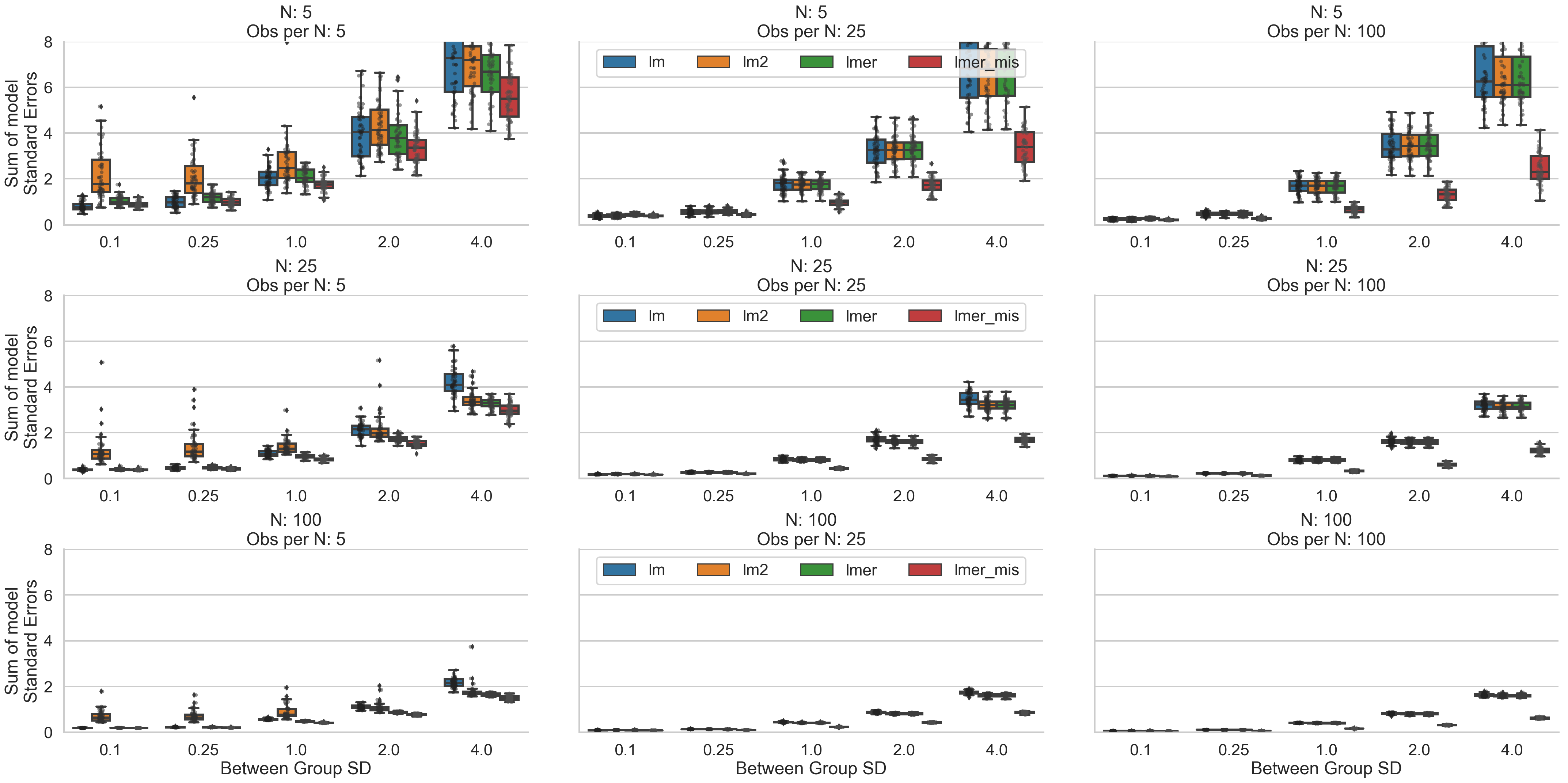
- Sum of Model Standard Errors - this and the next measure are more related to the inferences we want to make on our parameters. SE and the associated confidence intervals tell us the total amount of variance around our estimates given this particular modeling strategy. Once again, we could have computed the average, but like above, the sum gives us the total variance across all our parameters.
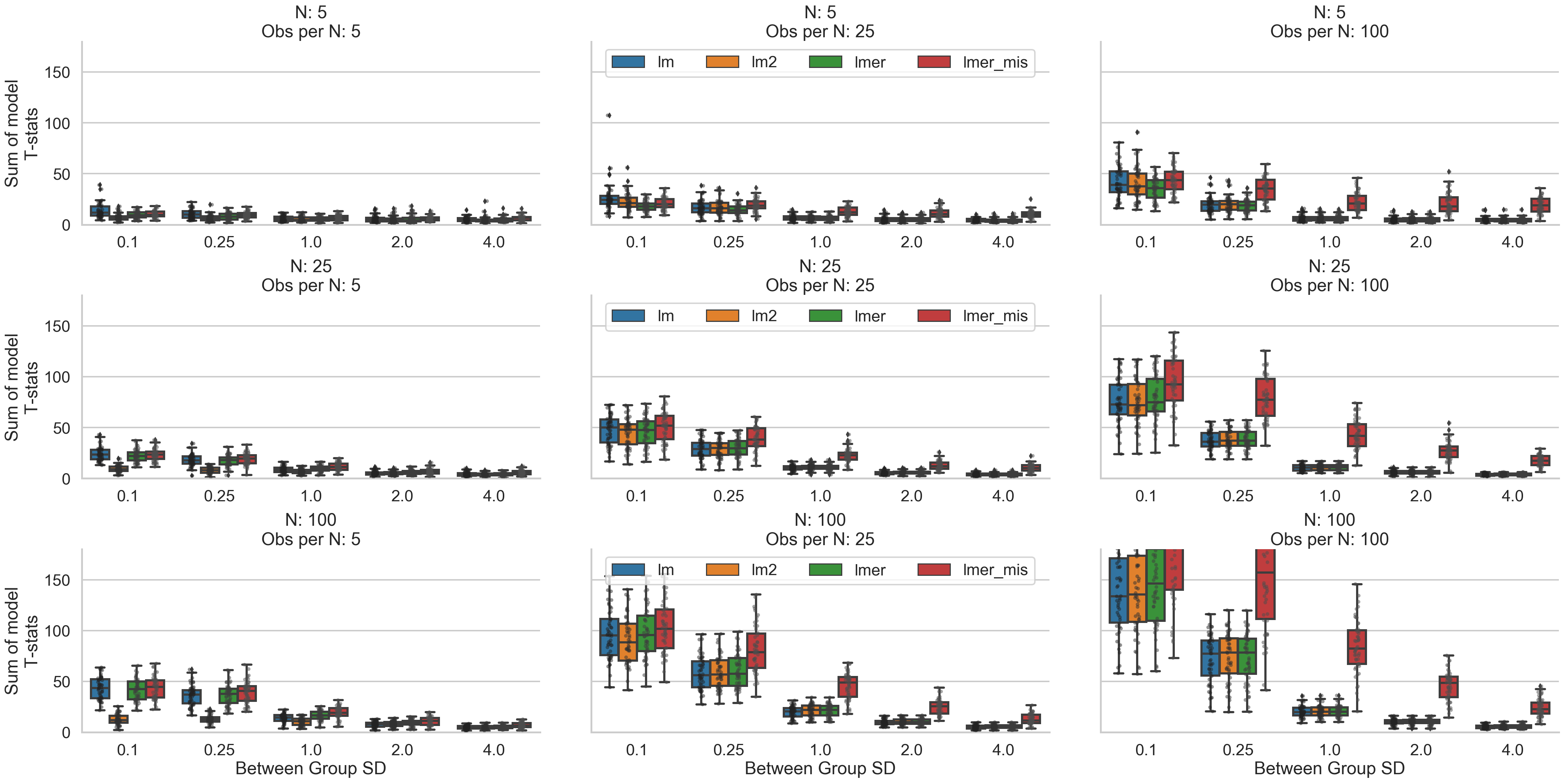
- Sum of Model T-statistics - this is the sum of the absolute value of the t-statistics of our model estimates. This gives us a sense of how likely we would be to walk away with the inference that there is a statistically significant relationship between our independent variables and dependent variable. All else being equal, larger t-stats generally mean smaller p-values so we can build an intuition about how sensitive our modeling strategy is to tell us “yup this is a statistically significant effect.”
Multi-level models
Let’s begin with fitting a multi-level model specifying the complete set of all possible parameters we can estimate. This has the effect of letting each individual have their own set of regression estimates while still treating these estimates as coming from a common distribution. You can see below we can recover the parameters pretty well and as we expect all our are results are “significant.”
# Fit lmer with random intercepts, slopes, and their correlations
lmer = Lmer(formula + '+ (IV1 + IV2 + IV3 | Group)',data=data)
lmer.fit(summarize=False)
lmer.coefs
print(f"Absolute Error of Coef Recovery: {diffs(betas, lmer.coefs['Estimate'])}")
print(f"Sum of Model Standard Errors: {lmer.coefs['SE'].sum()}")
print(f"Sum of Model T statistics: {lmer.coefs['T-stat'].abs().sum()}")
| Estimate | 2.5_ci | 97.5_ci | SE | DF | T-stat | P-val | Sig | |
|---|---|---|---|---|---|---|---|---|
| (Intercept) | 0.146146 | 0.072889 | 0.219402 | 0.037377 | 49.105624 | 3.910072 | 2.831981e-04 | *** |
| IV1 | 0.800926 | 0.720934 | 0.880917 | 0.040813 | 49.575279 | 19.624452 | 5.065255e-25 | *** |
| IV2 | 0.964310 | 0.874273 | 1.054347 | 0.045938 | 48.977731 | 20.991603 | 3.900389e-26 | *** |
| IV3 | 0.418673 | 0.336092 | 0.501255 | 0.042134 | 49.064194 | 9.936621 | 2.449657e-13 | *** |
Absolute Error of Coef Recovery: 0.10582723675727804
Sum of Model Standard Errors: 0.16626160033359066
Sum of Model T statistics: 54.46274837271574
Next, let’s see what happens when we fit a multi-level model with the simplest possible “random effects” structure. Notice that by not letting each individual be free to have their own estimates (aside from their own mean/intercept), our coefficient recovery drops a little bit, but our t-statistics increase dramatically. This looks to be driven by the fact that the variance estimates of the coefficients (standard errors) are quite a bit smaller. All else being equal, we would be much more likely to identify “significant” relationships using a simpler, or in this case, “misspecified” multi-level model, since we know that the data were generated such that each individual did in fact, have different BLUPs.
# Fit lmer with random-intercepts only
lmer_mis = Lmer(formula + '+ (1 | Group)',data=data)
lmer_mis.fit(summarize=False)
lmer_mis.coefs
print(f"Absolute Error of Coef Recovery: {diffs(betas, lmer_mis.coefs['Estimate'])}")
print(f"Sum of Model Standard Errors: {lmer_mis.coefs['SE'].sum()}")
print(f"Sum of Model T statistics: {lmer_mis.coefs['T-stat'].abs().sum()}")
| Estimate | 2.5_ci | 97.5_ci | SE | DF | T-stat | P-val | Sig | |
|---|---|---|---|---|---|---|---|---|
| (Intercept) | 0.153057 | 0.077893 | 0.228221 | 0.038350 | 49.009848 | 3.991084 | 2.195726e-04 | *** |
| IV1 | 0.800550 | 0.757763 | 0.843338 | 0.021831 | 2477.919857 | 36.670958 | 1.443103e-235 | *** |
| IV2 | 0.946433 | 0.902223 | 0.990644 | 0.022557 | 2473.820894 | 41.957498 | 4.899264e-291 | *** |
| IV3 | 0.403981 | 0.361007 | 0.446954 | 0.021926 | 2465.536399 | 18.424992 | 3.968080e-71 | *** |
Absolute Error of Coef Recovery: 0.1311098578975485
Sum of Model Standard Errors: 0.10466304433776347
Sum of Model T statistics: 101.04453264690632
Cluster-robust models
Next, let’s evaluate the cluster-robust-error modeling approach. Remember, this involves estimating a single regression model to obtain coefficient estimates, but then applying a correction factor to the SEs, and thereby the t-statistics to adjust our inferences. It looks like our coefficient recovery is about the same as our simple multi-level model above, but our inferences are far more conservative due to the larger standard-errors and smaller t-statistics. In fact, these are even a bit more conservative than the fully specified multi-level model we estimated first.
# Fit clustered errors LM
lm = Lm(formula,data=data)
lm.fit(robust='cluster',cluster='Group',summarize=False)
lm.coefs
print(f"Absolute Error of Coef Recovery: {diffs(betas, lm.coefs['Estimate'])}")
print(f"Sum of Model Standard Errors: {lm.coefs['SE'].sum()}")
print(f"Sum of Model T statistics: {lm.coefs['T-stat'].abs().sum()}")
| Estimate | 2.5_ci | 97.5_ci | SE | DF | T-stat | P-val | Sig | |
|---|---|---|---|---|---|---|---|---|
| Intercept | 0.153013 | 0.075555 | 0.230470 | 0.038481 | 46 | 3.976365 | 2.453576e-04 | *** |
| IV1 | 0.802460 | 0.712104 | 0.892815 | 0.044888 | 46 | 17.876851 | 0.000000e+00 | *** |
| IV2 | 0.945528 | 0.851538 | 1.039518 | 0.046694 | 46 | 20.249556 | 0.000000e+00 | *** |
| IV3 | 0.405163 | 0.313841 | 0.496485 | 0.045368 | 46 | 8.930504 | 1.307510e-11 | *** |
Absolute Error of Coef Recovery: 0.13278703905990247
Sum of Model Standard Errors: 0.17543089877808005
Sum of Model T statistics: 51.03327490657406
Two-stage-regression
Lastly, let’s use the two-stage-regression approach. We’ll fit a separate regression to each of our 50 people and then compute another regression on those 50 coefficients. In this simple example, we’re really just computing a one-sample t-test on these 50 coefficients. Notice that our coefficient recovery is a tiny bit better than our fully-specified multi-level model and our inferences (based on T-stats and SEs) would largely be similar. This suggests that for this particular dataset we could have gone with either strategy and walked away with the same inference.
# Fit two-stage OLS
lm2 = Lm2(formula,data=data,group='Group')
lm2.fit(summarize=False)
lm2.coefs
print(f"Absolute Error of Coef Recovery: {diffs(betas, lm2.coefs['Estimate'])}")
print(f"Sum of Model Standard Errors: {lm2.coefs['SE'].sum()}")
print(f"Sum of Model T statistics: {lm2.coefs['T-stat'].abs().sum()}")
| Estimate | 2.5_ci | 97.5_ci | SE | DF | T-stat | P-val | Sig | |
|---|---|---|---|---|---|---|---|---|
| (Intercept) | 0.144648 | 0.070338 | 0.218958 | 0.036978 | 49 | 3.911745 | 2.822817e-04 | *** |
| IV1 | 0.796758 | 0.716781 | 0.876736 | 0.039798 | 49 | 20.019944 | 0.000000e+00 | *** |
| IV2 | 0.971252 | 0.878498 | 1.064005 | 0.046156 | 49 | 21.042892 | 0.000000e+00 | *** |
| IV3 | 0.424135 | 0.339132 | 0.509138 | 0.042299 | 49 | 10.027041 | 1.840750e-13 | *** |
Absolute Error of Coef Recovery: 0.09216204521686983
Sum of Model Standard Errors: 0.16523098907361963
Sum of Model T statistics: 55.00162203260664
Simulating a universe.
Now, this was only one particular dataset with a particular size and particular level of between-person variability. Remember the dimensions outlined above? The real question we want to answer is how these different modeling strategies vary with respect to each of those dimensions. So let’s expand our simulation here. Let’s generate a “grid” of settings such that we simulate every combination of dimensions we can in a reasonable amount of time. Here’s the grid we’ll try to simulate:
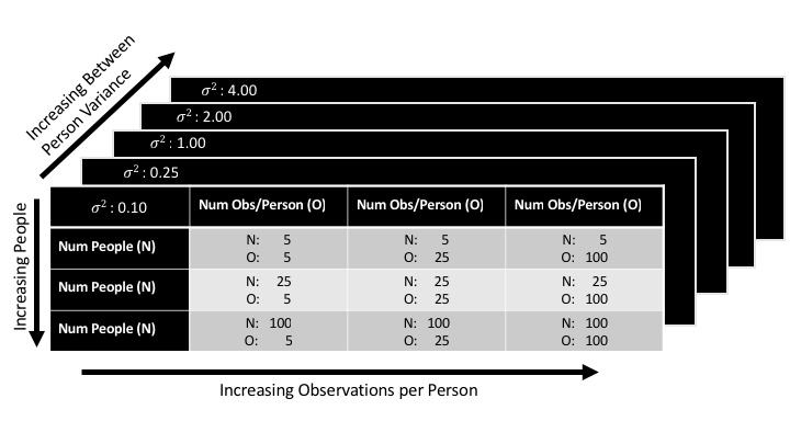
Going down the rows we’ll vary dimension 1 the sample size of the units we’re making inferences over (number of people) from 5 -> 100. Going across columns we’ll vary dimension 2, the sample size of the units nested within the units we’re making inferences over (number of observations per person) from 5 -> 100. Going over the z-plane we’ll vary dimension 3 the variance between the units we’re making inferences over (between-person variability) from 0.10 -> 4 standard deviations.
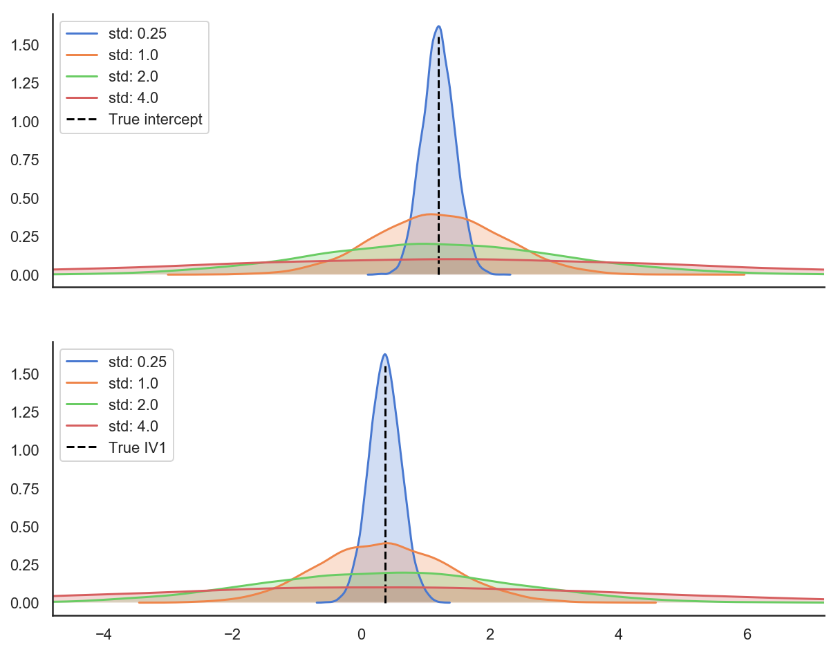
Since varying dimension 1 and dimension 2 should make intuitive sense (they’re different aspects of the sample size of our data) let’s explore what varying dimension 3 looks like. Here are plots illustrating how changing our between person variance influences coefficients. Each figure below depicts a distribution of person level coefficients; these are the BLUPs we discussed above. When simulating a dataset with two parameters described by an intercept and a slope (IV1), notice how each distribution is centered on the true value of the parameter, but the width of the distribution increases as we increase the between-group variance. These distributions are the distributions that our person level parameters come from. So while they average out to be the same value, they are increasingly dispersed around that value. As these distributions become wider it becomes more challenging to recover the true coefficients of the data if a dataset is too small, as models need more data in order to stabilize their estimates.
For the sake of brevity I’ve removed the plotting code for the figures below, but am happy to share them on request.
Setting it up
The next code block sets up this parameter grid and defines some helper functions to compute the metrics defined above. Since this simulation took about ~50 minutes to run on a 2015 quad-core Macbook Pro, I also defined some functions to save each simulation to a csv file.
# Define the parameter grid
nsim = 50 # Number of simulated datasets per parameter combination
num_grps = [10, 30, 100] # Number of "clusters" (i.e. people)
obs_grp = [5, 25, 100] # Number of observations per "cluster"
grp_sigmas = [.1, .25, 1., 2., 4.] # Between "cluster" variance
num_coef = 3 # Number of terms in the regression equation
noise_params = (0, 1) # Assume each cluster has normally distributed noise
seed = 0 # to repeat this simulation
formula = 'DV ~ IV1 + IV2 + IV3' # The model formula

# Define some helper functions. diffs() was used above examining each model in detail
def diffs(a, b):
    """Absolute error"""
    return np.sum(np.abs(a - b))

def calc_model_err(model_type, formula, betas, data):
    """
    Fit a model type to data using pymer4. Return the absolute error of the model's
    coefficients, the sum of the model's standard errors, and the sum of the model's
    t-statistics. Also log if the model failed to converge in the case of lme4.
    """

    if model_type == 'lm':
        model = Lm(formula, data=data)
        model.fit(robust='cluster',cluster='Group',summarize=False)
    elif model_type == 'lmer':
        model = Lmer(formula + '+ (IV1 + IV2 + IV3 | Group)',data=data)
        model.fit(summarize=False, no_warnings=True)
    elif model_type == 'lmer_mis':
        model = Lmer(formula + '+ (1 | Group)',data=data)
        model.fit(summarize=False, no_warnings=True)
    elif model_type == 'lm2':
        model = Lm2(formula,data=data,group='Group')
        model.fit(n_jobs = 2, summarize=False)

    coef_diffs = diffs(betas, model.coefs['Estimate'])
    model_ses = model.coefs['SE'].sum()
    model_ts = model.coefs['T-stat'].abs().sum()
    if (model.warnings is None) or (model.warnings == []):
        model_success = True
    else:
        model_success = False

    return coef_diffs, model_ses, model_ts, model_success, model.coefs

def save_results(err_params, sim_params, sim, model_type, model_coefs, df, coef_df, save=True):

    """Aggregate and save results using pandas"""

    model_coefs['Sim'] = sim
    model_coefs['Model'] = model_type
    model_coefs['Num_grp'] = sim_params[0]
    model_coefs['Num_obs_grp'] = sim_params[1]
    model_coefs['Btwn_grp_sigma'] = sim_params[2]

    coef_df = coef_df.append(model_coefs)

    dat = pd.DataFrame({
            'Model': model_type,
            'Num_grp': sim_params[0],
            'Num_obs_grp': sim_params[1],
            'Btwn_grp_sigma': sim_params[2],
            'Coef_abs_err': err_params[0],
            'SE_sum': err_params[1],
            'T_sum': err_params[2],
            'Fit_success': err_params[3],
            'Sim': sim
        },  index = [0])

    df = df.append(dat,ignore_index=True)
    if save:
        df.to_csv('./sim_results.csv',index=False)
        coef_df.to_csv('./sim_estimates.csv')
    return df, coef_df

# Run it
results = pd.DataFrame()
coef_df = pd.DataFrame()
models = ['lm', 'lm2', 'lmer', 'lmer_mis']
for N in num_grps:
    for O in obs_grp:
        for S in grp_sigmas:
            for I in range(nsim):
                data, blups, betas = simulate_lmm(O, num_coef, N, grp_sigmas=S, noise_params=noise_params)
                for M in models:
                    c, s, t, success, coefs, = calc_model_err(M, formula, betas, data)
                    results, coef_df = save_results([c,s,t, success], [N,O,S], I, M, coefs, results, coef_df)
Results
For the sake of brevity I’ve removed the plotting code for the figures below, but am happy to share them on request!
Coefficient Recovery
Ok, let’s take first take a look at our coefficient recovery. If we look from the top left of the grid to the bottom right the first thing to jump out is that when we increase our overall sample size (number of clusters * number of observations per cluster), and our between cluster variability is medium to low, all model types do a similarly good job of recovering the true data generating coefficients. In other words, under good conditions (lots of data that isn’t too variable) we can’t go wrong picking any of the analysis strategies. In the converse, going from bottom left to top right, when between cluster variability is high, we quickly see the importance of having more clusters rather than more observations per cluster; without enough clusters to observe, even a fully specified multi-level model does a poor job of recovering the true coefficients.
When we have small to medium sized datasets and lots of between-cluster variability all models tend to do a poor job of recovering the true coefficients. Interestingly, having particularly few observations per cluster (left-most column) disproportionately affects two-stage-regression estimation (orange boxplots). This is consistent with Gelman, 2005 who suggests that with few per cluster observations, the first-level OLS estimates are pretty poor with high-variance and there are none of the multi-level modeling benefits to help offset the situation. This situation also seems to favor fully-specified multi-level models the most (green boxplots), particularly when between cluster variability is high. It’s interesting to note that cluster-robust, and misspecified (simple) multi-level models seem to perform similarly in this situation.
In medium data situations (middle column) cluster-robust models seem to do a slightly worse job across the board of recovering coefficients. This is most likely due to the fact that the estimates completely ignore the clustered nature of the data and have no smoothing/regularization applied to them either through averaging (in the case of the two-stage-regression models) or through random-effects estimation (in the case of the multi-level models).
Finally, in the high observations per cluster situation (right-most column), all models seem to perform rather similarly suggesting that each modeling strategy is about as good as any other when we densely sampling the unit of interest (increasing number of observations per cluster) even if the desire is to make inferences about the clusters themselves.
Making Inferences (SEs + T-stats)
Next, let’s look at both standard errors and t-statistics to see how our inferences might vary. The effect of increased between cluster variance has a very notable effect on SEs and t-stats values generally making it less likely to identify a statistically significant relationship regardless of the size of the data. Interestingly, what two-stage-regression models exhibit in terms of poorer coefficient recovery in situations with few observations per cluster, they make up for with higher standard error estimates. We can see that their t-statistics are low in these situations suggesting that in these situations this approach may tip the scales towards lower false-positive, higher false-negative inferences. However, unlike other model types, they do not necessarily benefit from more clusters overall (bottom left panel) and run the risk of an inflated level of false negatives. Misspecified multilevel models seem to have the opposite properties: they have higher t-stats and lower SEs in most situations with medium to high between-cluster variability and benefit the most from situations with a high number of observations per cluster. This suggests they might run the risk of introducing more false positives in situations where other models may behave more conservatively, but also may be more sensitive to detecting true relationships in the face of high between-cluster variance. They also seem to benefit most from increasing observations within cluster. Inferences from cluster-robust and full-specified multi-level models seem to be largely comparable which is consistent with the proliferate use of both these model types across multiple literatures.
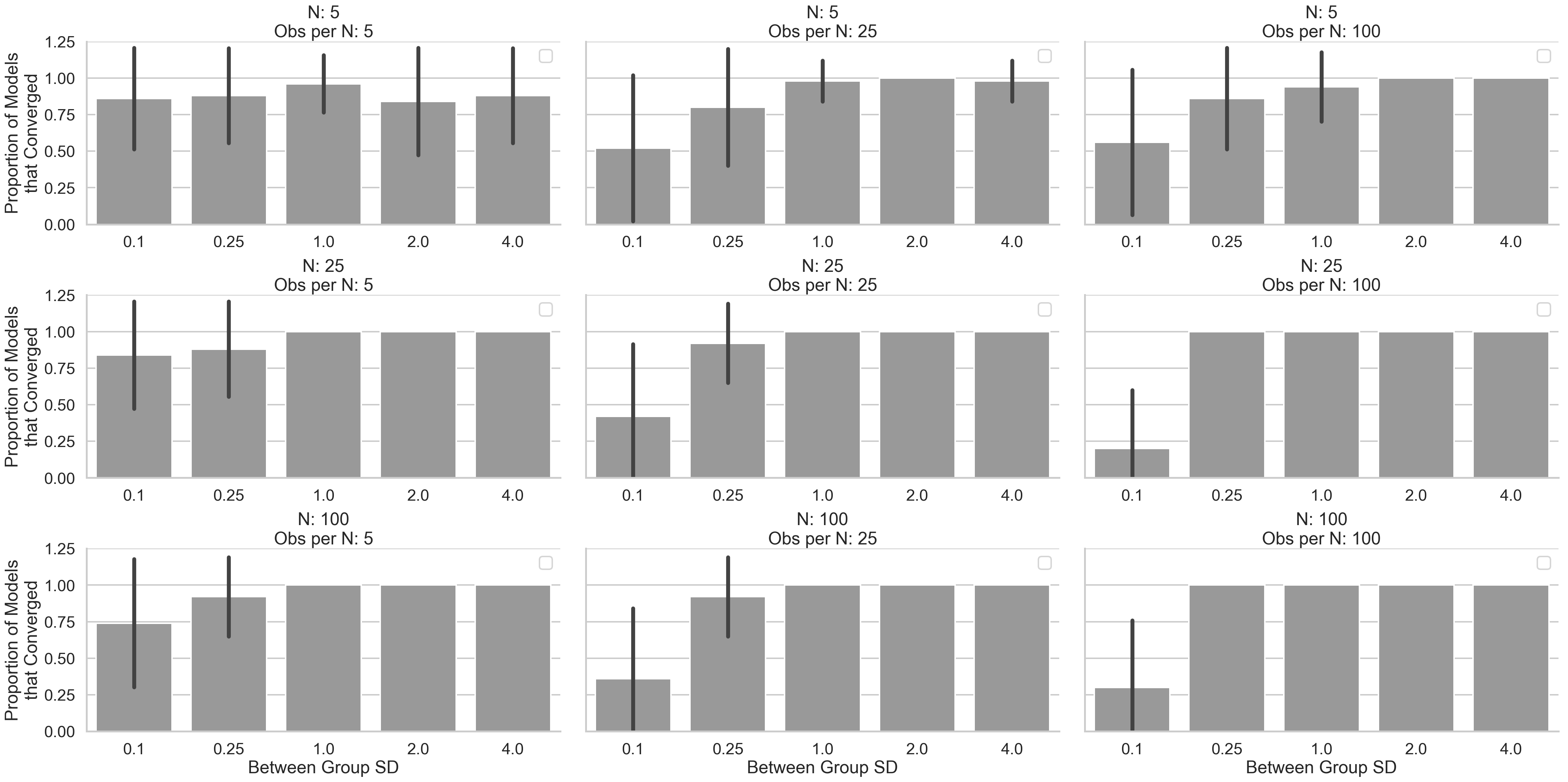
Bonus: When fully-specified multi-level models fail
Finally, we can take a brief look at what situations most often cause convergence failures for our fully-specified multi-level models (note: the simple multi-level models examined earlier never failed to converge in these simulations). In general, this seems to occur when between cluster variability is low, or the number of observations per cluster is very small. This makes sense because even though the data were generated in a multi-level manner, clusters are quite similar and simplifying models by discarding terms which try to model variance that may not be exhibited by the data in a meaningful way (e.g. dropping “random-slopes”) achieve better estimation overall. In other words, the model may be trying to fit a variance parameter that is small enough to cause it to run out of optimizer iterations before it reaches a suitably small change in error. This is like trying to find the lowest point on a “hill” that has a very shallow declining slope by comparing the height of your current step to the height of your previous step.
Conclusions
So what have we learned? Here are some intuitions that I think this exercise has helped flesh out:
- Reserve two-stage-regression for situations when there are enough observations per cluster. This is because modeling each cluster separately without any type of smoothing/regularization/prior imposed by multi-level modeling, produces poor first-level estimates in these situations.
- Be careful using misspecified/simple multi-level models. While they may remove some of the complexity involved in specifying the “random effects” part of the model, and they converge pretty much all the time, they are more likely to lead to statistically significant inferences relative to other approaches (all else being equal). This may be warranted if your data don’t exhibit enough between-cluster variance. It may be generally preferable then to specify a model structure that accounts for variance confounded with predictors of interest (Barr et al, 2013) (i.e. dropping the correlation term between a random intercept and random slope rather than dropping the random slope), in other words the most “maximal” structure you can get away with, with respect to the inferences you want to make of your data.
- Cluster-robust models appear to be an efficient solution if your primary goal is making inferences and you can live with coefficient estimates that are a bit less accurate than other approaches. These are harder to specify if there are multiple levels of clustering in the data (e.g. survey responses within-person, within-city, within-state, etc) or if accounting for item-level effects are important (Baayen et al, 2008). However, there are techniques to incorporate two-way or multi-way cluster-robust errors and such approaches are reasonably common in economics. This lecture and this paper discuss these approaches further. Pymer4 used for this post only implements one-way clustering.
- Consider using two-stage-regression or cluster-robust errors1 instead of misspecified multi-level models as your inferences maybe be largely similar to fully-specified multi-level models that converge successfully. This may not be true if item-level variance or multiple-levels of clustering need to be taken into account, but for relatively straight forward cases illustrated in this post, they seem to fair just fine.
- Generally, simulations can be helpful ways to build statistical intuitions especially if the background mathematics feels daunting. This is has been one of my preferred approaches for learning statistical concepts in more depth and has made reading literature heavy on mathematical formalisms far more approachable.
Caveats and cautions
I don’t want to end this post with the feeling that we’ve figured everything out and are expert analysts now, but rather appreciate that there are some limitations to this exercise that are worth keeping in mind. While we can build some general intuitions, there are conditions under which these intuitions may not always hold and it’s incredibly important to be aware of them:
- In many ways, the data generated in these simulations were “ideal” for playing around with these different approaches. Data points were all on the same scale, came from a normal distribution with known means and variances, contained no missing data points, and adhered to other underlying assumptions of these statistical approaches not discussed.
- Similarly, I built-in “real relationships” into the data and then tried to recover them. I made mention of false-positives and negatives throughout the post, but I did not formally estimate the false-positive or false-negative rate for any of these approaches. Again this was by design to leave you with some general intuitions, but there exist several papers that utilize this approach to more explicitly defend the use of certain inference techniques (e.g. Luke, 2017).
- The space of parameters we explored (i.e. the different “dimensions” of our data) spanned a range I thought reasonably covered a variety of datasets often collected in empirical social science laboratory studies. In the real world, data are far messier and increasingly, far larger. More data is almost always better, particularly if it’s of high quality, but what constitutes quality can be very different based on the inferences one wants to make. Sometimes high variability between clusters is desirable, other times densely sampling a small set of clusters is more important. These factors will vary based on the questions one is trying to answer.
- The metrics I chose to evaluate each model with are simply the ones that I wanted to know about. There are certainly other metrics that could be more or less informative based on what intuitions you would like to build. For example, what is the prediction accuracy of each model?
Conclusion
I hope this was useful for some folks out there and even if it wasn’t, it certainly helped me build some intuitions about the different analysis strategies that are available. Moreover, I hope if nothing else, this might motivate people who feel like they have limited formal training in statistics/machine-learning to take a more tinker/hacker approach to their own learning. I remember when as a kid, breaking things and taking them apart was one of my favorite ways to learn about how things worked. With the mass availability of free and open-source tools like scientific Python and R, I see no reason why statistical education can’t be the same.
Appendix
This is a nice quick guide that defines much of the terminology across different fields and reviews a lot of the concepts covered here (plus more) in a much more pithy way. For those interested, p-values for multi-level models were computed using the lmerTest R package using Satterthwaite approximation for degrees of freedom calculation; note that based on the random-effects structure specified, these degrees of freedom can change dramatically. P-values for other model types were computed using a standard t-distribution, but pymer4 also offers non-parametric permutation testing and boot-strapped confidence intervals for other styles of inference. At the time of this writing, fitting two-stage-regression models is only available in development branch on github, but should be incorporated in a new release in the future.
Notes and Corrections
*In a previous version of this post, this approach was mistakenly called two-stage-least-squares (2SLS). 2SLS is a formal name for a completely different technique which falls under the broader scope of instrumental variable estimation. This confusion is because the two-stage-regression approach discussed above technically does employ “two-stages” of ordinary-least-squares estimation, yet this is not what 2SLS is in the literature. Thanks to Jonas Oblesser for pointing this out and Stephen John Senn for appropriate terminology that is in fact consistent across medical and fMRI literatures.↩
1. While in this post (and often in the literature) two-stage, or even multi-level modeling and cluster-robust inference are seen as two different possible analytic strategies another possibility involves combining these approaches. That is, using a multi-level model or two-stage-regression to obtain coefficient estimates, and then computing robust-standard errors on the highest-level coefficients when performing inference. Thanks to James E. Pustejovsky for bringing up this often overlooked option.↩