Note
Go to the end to download the full example code
1. Basic Usage Guide
pymer4 comes with sample data for testing purposes which we’ll utilize for most of the tutorials.
This sample data has:
Two kinds of dependent variables: DV (continuous), DV_l (dichotomous)
Three kinds of independent variables: IV1 (continuous), IV2 (continuous), IV3 (categorical)
One grouping variable for multi-level modeling: Group.
Let’s check it out below:
# import some basic libraries
import os
import pandas as pd

# import utility function for sample data path
from pymer4.utils import get_resource_path

# Load and checkout sample data
df = pd.read_csv(os.path.join(get_resource_path(), "sample_data.csv"))
print(df.head())
   Group   IV1  DV_l         DV       IV2  IV3
0      1  20.0     0   7.936508  4.563492  0.5
1      1  20.0     0  15.277778  0.000000  1.0
2      1  20.0     1   0.000000  0.000000  1.5
3      1  20.0     1   9.523810  0.000000  0.5
4      1  12.5     0   0.000000  0.000000  1.0
Standard regression models
Fitting a standard regression model is accomplished using the Lm model class in pymer4. All we need to do is initialize a model with a formula, some data, and call its .fit() method.
By default the output of .fit() has been formated to be a blend of summary() in R and .summary() from statsmodels. This includes metadata about the model, data, and overall fit as well as estimates and inference results of model terms.
# Import the linear regression model class
from pymer4.models import Lm

# Initialize model using 2 predictors and sample data
model = Lm("DV ~ IV1 + IV2", data=df)

# Fit it
print(model.fit())
Formula: DV~IV1+IV2

Family: gaussian         Estimator: OLS

Std-errors: non-robust  CIs: standard 95%       Inference: parametric

Number of observations: 564      R^2: 0.512      R^2_adj: 0.510

Log-likelihood: -2527.681        AIC: 5061.363   BIC: 5074.368

Fixed effects:

           Estimate  2.5_ci  97.5_ci     SE   DF  T-stat  P-val  Sig
Intercept     1.657  -4.107    7.422  2.935  561   0.565  0.573
IV1           0.334  -0.023    0.690  0.181  561   1.839  0.066    .
IV2           0.747   0.686    0.807  0.031  561  24.158  0.000  ***
All information about the model as well as data, residuals, estimated coefficients, etc are saved as attributes and can be accessed like this:
# Print model AIC
print(model.AIC)
5061.3629635837815
# Look at residuals (just the first 10)
print(model.residuals[:10])
[-3.79994762  6.94860187 -8.32917613  1.19463387 -5.8271851  -6.88457421
  0.40673658  9.77173122 -7.33135842 -7.37107236]
A copy of the dataframe used to estimate the model with added columns for residuals and fits are are available at model.data. Residuals and fits can also be directly accessed using model.residuals and model.fits respectively
# Look at model data
print(model.data.head())
   Group   IV1  DV_l         DV       IV2  IV3       fits  residuals
0      1  20.0     0   7.936508  4.563492  0.5  11.736456  -3.799948
1      1  20.0     0  15.277778  0.000000  1.0   8.329176   6.948602
2      1  20.0     1   0.000000  0.000000  1.5   8.329176  -8.329176
3      1  20.0     1   9.523810  0.000000  0.5   8.329176   1.194634
4      1  12.5     0   0.000000  0.000000  1.0   5.827185  -5.827185
This makes it easy to assess overall model fit visually, for example using seaborn
# import dataviz
import seaborn as sns

# plot model predicted values against true values
sns.regplot(x="fits", y="DV", data=model.data, fit_reg=True)
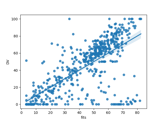
<Axes: xlabel='fits', ylabel='DV'>
Robust and WLS estimation
Lm models can also perform inference using robust-standard errors or perform weight-least-squares (experimental feature) for models with categorical predictors (equivalent to Welch’s t-test).
# Refit previous model using robust standard errors
print(model.fit(robust="hc1"))
Formula: DV~IV1+IV2

Family: gaussian         Estimator: OLS

Std-errors: robust (hc1)        CIs: standard 95%       Inference: parametric

Number of observations: 564      R^2: 0.512      R^2_adj: 0.510

Log-likelihood: -2527.681        AIC: 5061.363   BIC: 5074.368

Fixed effects:

           Estimate  2.5_ci  97.5_ci     SE   DF  T-stat  P-val  Sig
Intercept     1.657  -3.429    6.744  2.590  561   0.640  0.522
IV1           0.334  -0.026    0.693  0.183  561   1.823  0.069    .
IV2           0.747   0.678    0.815  0.035  561  21.444  0.000  ***
# Since WLS is only supported with 2 groups for now, filter the data first
df_two_groups = df.query("IV3 in [0.5, 1.0]").reset_index(drop=True)

# Fit new a model using a categorical predictor with unequal variances (WLS)
model = Lm("DV ~ IV3", data=df_two_groups)
print(model.fit(weights="IV3"))
Formula: DV~IV3

Family: gaussian         Estimator: WLS

Std-errors: non-robust  CIs: standard 95%       Inference: parametric

Number of observations: 376      R^2: 0.999      R^2_adj: 0.999

Log-likelihood: -532.518         AIC: 1069.036   BIC: 1076.896

Fixed effects:

           Estimate  2.5_ci  97.5_ci     SE       DF  T-stat  P-val  Sig
Intercept    45.647  35.787   55.507  5.015  373.483   9.103  0.000  ***
IV3          -2.926 -15.261    9.410  6.273  373.483  -0.466  0.641
Multi-level models
Fitting a multi-level model works similarly and actually just calls lmer or glmer in R behind the scenes. The corresponding output is also formatted to be very similar to output of summary() in R.
# Import the lmm model class
from pymer4.models import Lmer

# Initialize model instance using 1 predictor with random intercepts and slopes
model = Lmer("DV ~ IV2 + (IV2|Group)", data=df)

# Fit it
print(model.fit())
Model failed to converge with max|grad| = 0.00358015 (tol = 0.002, component 1)

Linear mixed model fit by REML [’lmerMod’]
Formula: DV~IV2+(IV2|Group)

Family: gaussian         Inference: parametric

Number of observations: 564      Groups: {'Group': 47.0}

Log-likelihood: -2249.281        AIC: 4510.562

Random effects:

                 Name      Var     Std
Group     (Intercept)  203.390  14.261
Group             IV2    0.136   0.369
Residual               121.537  11.024

               IV1  IV2   Corr
Group  (Intercept)  IV2 -0.585

Fixed effects:

             Estimate  2.5_ci  97.5_ci     SE      DF  T-stat  P-val  Sig
(Intercept)    10.300   4.806   15.795  2.804  20.183   3.674  0.001   **
IV2             0.682   0.556    0.808  0.064  42.402  10.599  0.000  ***
Similar to Lm models, Lmer models save details in model attributes and have additional methods that can be called using the same syntax as described above.
# Get population level coefficients
print(model.coefs)
              Estimate    2.5_ci    97.5_ci  ...     T-stat         P-val  Sig
(Intercept)  10.300430  4.805524  15.795335  ...   3.674034  1.487605e-03   **
IV2           0.682128  0.555987   0.808268  ...  10.598847  1.706855e-13  ***

[2 rows x 8 columns]
# Get group level coefficients (just the first 5)
# Each row here is a unique intercept and slope
# which vary because we parameterized our rfx that way above
print(model.fixef.head(5))
   (Intercept)       IV2
1     4.482095  0.885138
2    17.991023  0.622143
3     8.706144  0.838055
4    10.143487  0.865341
5    10.071328  0.182101
# Get group level deviates from population level coefficients (i.e. rfx)
print(model.ranef.head(5))
   X.Intercept.       IV2
1     -5.818335  0.203011
2      7.690593 -0.059985
3     -1.594286  0.155927
4     -0.156943  0.183213
5     -0.229102 -0.500026
Lmer models also have some basic plotting abilities that Lm models do not
# Visualize coefficients with group/cluster fits overlaid ("forest plot")
model.plot_summary()
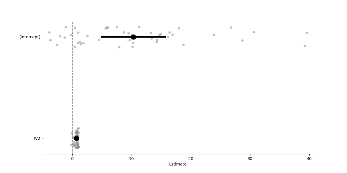
<Axes: xlabel='Estimate'>
Plot coefficients for each group/cluster as separate regressions
model.plot("IV2", plot_ci=True, ylabel="predicted DV")
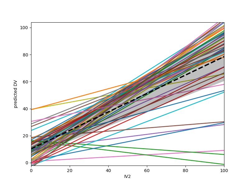
<Axes: xlabel='IV2', ylabel='predicted DV'>
Because Lmer models rely on R, they have also some extra arguments to the .fit() method for controlling things like optimizer behavior, as well as additional methods such for post-hoc tests and ANOVAs. See tutorial 2 for information about this functionality.
Two-stage summary statistics models
Fitting Lm2 models are also very similar
# Import the lm2 model class
from pymer4.models import Lm2

# This time we use the 'group' argument when initializing the model
model = Lm2("DV ~ IV2", group="Group", data=df)

# Fit it
print(model.fit())
/home/runner/work/pymer4/pymer4/pymer4/stats.py:657: RuntimeWarning: invalid value encountered in scalar divide
  return 1 - (rss / tss)
Formula: DV~IV2

Family: gaussian

Std-errors: non-robust  CIs: standard 95%       Inference: parametric

Number of observations: 564      Groups: {'Group': 47}

Fixed effects:

           Estimate  2.5_ci  97.5_ci     SE  DF  T-stat  P-val  Sig
Intercept    14.240   4.891   23.589  4.644  46   3.066  0.004   **
IV2           0.614   0.445    0.782  0.084  46   7.340  0.000  ***
Like Lmer models, Lm2 models also store group/cluster level estimates and have some basic plotting functionality
# Get group level coefficients, just the first 5
print(model.fixef.head(5))
       Intercept       IV2
Group
1       3.039903  1.781832
2      23.388350  0.524852
3       4.904321  0.919913
4      23.304669  0.719425
5      18.378387 -0.256136
# Visualize coefficients with group/cluster fits overlaid ("forest plot")
model.plot_summary()
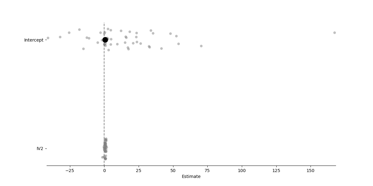
<Axes: xlabel='Estimate'>
Model Persistence
All pymer4 models can be saved and loaded from disk. Doing so will persist all model attributes and data i.e. anything accessible with the ‘.’ syntax. Models are saved and loaded using Joblib Therefore all filenames must end with .joblib. For Lmer models, an additional file ending in .rds will be saved in the same directory as the HDF5 file. This is the R model object readable in R using readRDS.
Prior to version 0.8.1 models were saved to HDF5 files using deepdish but this library is no longer maintained. If you have old models saved as .h5 or .hdf5 files you should use the same version of pymer4 that you used to estimate those models.
To persist models you can use the dedicated save_model and load_model functions from the pymer4.io module
# Import functions
from pymer4.io import save_model, load_model

# Save the Lm2 model above
save_model(model, "mymodel.joblib")
# Load it back up
model = load_model("mymodel.joblib")
# Check that it looks the same
print(model)
pymer4.models.Lm2(fitted=True, formula=DV~IV2, family=gaussian, group=Group)
Wrap Up
This was a quick overview of the 3 major model classes in pymer4. However, it’s highly recommended to check out the API to see all the features and options that each model class has including things like permutation-based inference (Lm and Lm2 models) and fine-grain control of optimizer and tolerance settings (Lmer models).